Two sales exports from two regions, or a product list and a price list that live in separate files. Copy-paste gets the job done once, then breaks the moment either file updates. Power Query solves that, but the single most common reason a combined dataset produces a wrong pivot table is picking the wrong combine operation at the start. Append and Merge are not interchangeable, and choosing wrongly can double your row count or leave half your columns blank — a mistake that is easy to spot at 200 rows and nearly invisible at 20,000.
The rule is short: Append stacks rows, Merge joins columns. If your second table has the same columns as the first with more records, you want Append. If your second table has different columns that describe the same entities, you want Merge. Everything below is the step-by-step for both, followed by the pivot table setup that makes the combined result usable.
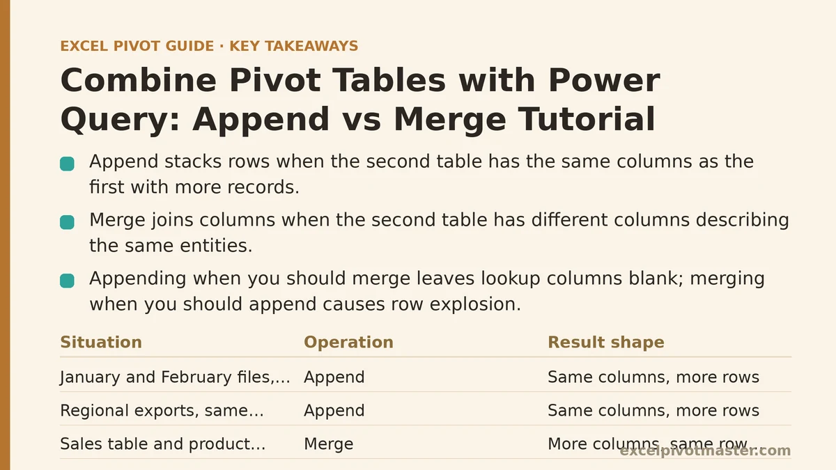
The Decision That Comes First
Before touching a single button, look at the shape of your two tables. The answer is usually obvious once you frame it as a question.
| Your situation | Operation | Result shape | Typical use case |
|---|---|---|---|
| January file and February file, identical columns | Append | Same columns, more rows | Monthly export stacking |
| Regional exports from separate systems, same schema | Append | Same columns, more rows | Consolidating branches or regions |
| Sales table and a product lookup table (SKU, category, cost) | Merge | More columns, same row count | Enriching transactions with attributes |
| Orders table and a customer master file | Merge | More columns, same row count | Adding customer segment, region, rep |
| Two tables where one is a subset of the other | Append (then dedupe) | Union of rows | Combining a current file with an archive |
| Two tables with different columns and no common key | Neither — fix the data first | N/A | Likely a schema or key problem |
If you append when you should merge, your pivot will show the lookup columns as blanks on half the rows. If you merge when you should append, you will get a repeated join of every row against every match — a row explosion that can turn 10,000 records into 400,000 in a single click.
Step 1: Load Both Sources Into Power Query as Separate Queries
The pivot table itself is not where the combining happens. Power Query builds a new table, you load that table to the workbook, and the pivot reads from it. Keeping the two raw sources as their own queries is what makes the whole thing refreshable later.
- Open a blank workbook or the workbook that will hold the final pivot.
- Go to Data → Get Data → From File → From Workbook (or From Text/CSV, From Table/Range, etc.) and point it at your first source. In the Navigator dialog, tick the table or sheet and choose Transform Data, not Load.
- Repeat for the second source. Again, Transform Data.
- In the Power Query Editor, rename both queries in the left-hand Queries pane to something meaningful —
Sales_JanandSales_Feb, for example. Double-click the query name to rename.
At this point you should have two queries, each ending with a set of steps on the right-hand Applied Steps pane. Nothing has been loaded to a worksheet yet, which is correct.
Check before moving on: Click each query and confirm the column headers are identical in spelling, case, and spacing. Customer ID, customer id, and CustomerID are three different columns to Power Query, and they will not stack cleanly in an Append.
Step 2A: Append — Stacking Rows From Two Same-Shape Tables
Append answers the question “what if these two tables were one long table?” The column count stays the same; only the number of rows grows.
The clicks
- With either query selected, go to Home → Append Queries → Append Queries as New.
- In the dialog, set the primary table to
Sales_Janand addSales_Febin the second slot. If you have three or more files, choose Three or more tables and add each one. - Click OK. Power Query creates a third query — rename it
Sales_All. - Expand the new query and scroll through. You should see January rows, then February rows underneath, with the same column headers across the whole set.
The three things that go wrong with Append
- Mismatched headers. If one file calls the column
Regionand the otherSales Region, the Append produces two separate columns, each half-populated. Fix the names in each source query first (right-click the header → Rename) so both queries match before appending. - Different column order. Order does not matter — Power Query matches by name, not position. You do not need to rearrange anything.
- Extra or missing columns. If February has a
Discountcolumn that January lacks, the append still works, but January rows show null inDiscount. Decide whether that is correct or whether January needs the column added.
When your files arrive one per month
The real advantage appears when files keep coming. Instead of appending two fixed queries, point Get Data → From Folder at a directory of monthly exports. Power Query reads every file in the folder matching your pattern, applies each one’s steps, and the combined query grows automatically as new files are dropped in. One refresh in Excel pulls in the new month with no manual steps.
Step 2B: Merge — Joining Columns From Two Tables That Share a Key
Merge answers a different question: “for each row here, what does the matching row in the other table say?” Row count should stay the same (unless the key is duplicated, covered below); column count grows.
The clicks
- Select the query that will be the left side of the join — typically your transactions or fact table, e.g.
Sales. - Go to Home → Merge Queries → Merge Queries as New.
- In the dialog, the top table is
Sales. In the bottom dropdown, choose the lookup table —Products. - Click the matching column in each table. If Sales has
ProductIDand Products hasProductID, clickProductIDon top andProductIDon the bottom. Both headers turn bold when selected. - Set the Join Kind. For a lookup, Left Outer is almost always right: keep every sales row, bring in matching product attributes, and leave nulls where no product match exists. Click OK.
- Power Query creates a new query. You will see a new column containing the word
Tablein every cell. Click the expand icon (two arrows pointing outward) in that column header. Untick Use original column name as prefix and select only the columns you want to bring across — for exampleCategoryandUnitCost. Click OK. - Rename the finished query
Sales_Enriched.
Join kinds, briefly
| Join kind | Keeps | When to use |
|---|---|---|
| Left Outer | All left rows, matched right columns | Standard enrichment — keep all transactions |
| Inner | Only rows with a match on both sides | Finding only valid, matched records |
| Left Anti | Only left rows with no match | Auditing unmatched transactions |
| Right Outer / Full Outer | All rows from right / from both sides | Rarely needed for pivot prep |
For pivot-table work, Left Outer is the default choice. It preserves every transaction and fills in attributes only where a lookup exists.
Watch for duplicate keys in the lookup table
This is the failure that silently triples your data. If the Products table contains the same ProductID twice, a Merge will produce two rows for every sales row that matches it. A pivot built on the result then sums every affected transaction twice. Before merging, check the lookup table:
- Select the key column and use Home → Remove Rows → Remove Duplicates in the lookup query if duplicates are a data error.
- If duplicates are legitimate (a product with multiple prices by date), you need a more specific join key — often a combination of two columns — rather than a plain one-column merge.
Step 3: Clean Up Columns Before Loading
Whichever operation you ran, your combined query still needs a pass before it goes to a pivot table.
- Set data types. Click the small icon at the left of each column header and set the type explicitly — Whole Number for IDs, Date for dates, Decimal Number for currency. Do this on every column. Unset types cause sorting errors and inconsistent totals in the pivot.
- Remove unused columns. Right-click → Remove Column on anything the pivot will not use. A leaner query refreshes faster.
- Rename for readability. The pivot field list will show whatever the column headers say.
Total Sales ($)reads better thanColumn7. - Check the row count. The status bar at the bottom of the Power Query Editor shows how many rows the current step contains. Compare that number against what you expect from the source. A sudden jump from 10,000 to 40,000 after a Merge is the duplicate-key problem above.
Step 4: Load the Result and Build the Pivot Table
- With your finished query selected, go to Home → Close & Load → Close & Load To…
- Choose Table and New Worksheet (or Existing Worksheet). This puts the cleaned, combined data on a sheet as a proper Excel Table.
- Select any cell in that loaded table and go to Insert → PivotTable. Because the source is an Excel Table rather than a fixed cell range, the pivot cache expands automatically as Power Query adds rows on refresh.
- Build your pivot normally. Row labels, values, filters — everything behaves as if you had typed the combined data yourself.
The important habit: never point the pivot at the raw source files directly. The pivot reads the loaded Power Query table, and that table is what refresh re-reads when the underlying files change.
The refresh sequence
When source data updates, the update has two stages. Press Data → Refresh All once. Power Query re-runs its steps, the loaded table updates, and the pivot reads the new rows — all in a single action. If you press only the pivot’s refresh (Alt+F5), you re-read the old loaded table without re-running Power Query, and new source files go unseen.
Append vs Merge: The Recovery Moves
If you have already built the wrong operation, undoing it is fast.
If you appended when you should have merged: The symptom is that your pivot shows lookup columns as mostly blanks. Delete the append query, revert to the two source queries, and run a Merge instead.
If you merged when you should have appended: The symptom is a row count far larger than your source records, and duplicated totals in the pivot. Check the lookup table for duplicate keys. Remove duplicates on the key, or find a composite key, then re-run the merge.
If you picked the wrong join kind: Open the merge query, find the Source step in Applied Steps, delete every step after it, and re-run Merge with the correct join kind. Changing the join kind after the fact means deleting and redoing the merge — Power Query does not offer a toggle once the step exists.
If duplicate rows appear after an Append: The two source files overlap — for example the February file accidentally includes January records. Add a step to the combined query: select the key column, Remove Duplicates.
A Short Checklist Before You Click Refresh All
- Both source queries renamed and free of mismatched header spellings.
- Append used only when the two tables have the same core columns.
- Merge used only when a shared key column exists and is reliable.
- Left Outer join kind selected for standard enrichment.
- Lookup table checked for duplicate keys.
- Data types set on every column in the final query.
- Row count compared against expected source count.
- Pivot table sourced from the loaded Power Query table, not the raw files.
What to Do Next
Open the two files you intend to combine and answer one question on paper: do they describe the same things (same columns, more records → Append) or related things (a shared key, different columns → Merge)? Write the answer down before opening Power Query.
Then work through it in this order:
- Load each source as its own query with Transform Data (do not Load directly).
- Normalize the column headers so key and shared columns match exactly.
- Run Append Queries as New or Merge Queries as New according to the answer above.
- Set data types, drop unused columns, and check the row count on the status bar.
- Close & Load To… a new worksheet as a Table.
- Insert the PivotTable from that table, then use Data → Refresh All — not just the pivot’s refresh — every time the source files change.
Get steps 1 through 3 right and the pivot table becomes a report that maintains itself. Get them wrong and no amount of refresh-clicking will fix a doubled total or a column of blanks.