Click on a cell inside a pivot table while building a formula, and Excel will not give you what you asked for. You expect =C7. You get =GETPIVOTDATA("Sum of Revenue",$A$3,"Region","West","Month","March"). This isn’t a bug, and it isn’t random — it’s a built-in setting that’s been quietly switched on by default for years, and most people never learn it exists until it starts breaking something.
Once you understand what triggers it, GETPIVOTDATA stops being a mystery and turns into a tool you can either use on purpose or shut off entirely. Below are the questions people ask most often once they notice it happening.
What exactly is GETPIVOTDATA doing?
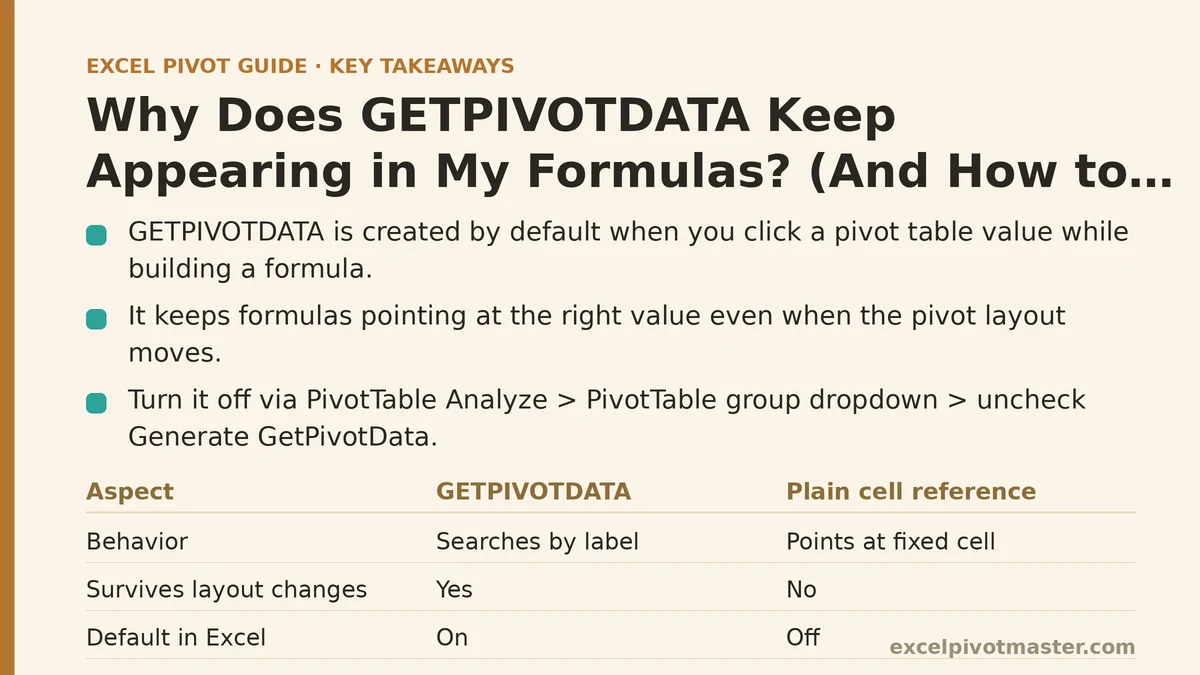
GETPIVOTDATA is a function that pulls a specific value out of a pivot table by describing what you want in words — which field, which row category, which column category — rather than by pointing at a fixed cell address. Instead of “give me whatever is in C7,” it says “give me the Sum of Revenue where Region is West and Month is March,” and it searches the pivot table’s structure to find that value wherever it currently lives.
That distinction matters because pivot tables move. Add a new region, sort the fields differently, or collapse a group, and the value that used to sit in C7 might now be sitting in C9. A plain cell reference would happily return whatever ends up in C7 after the shuffle, even if that’s the wrong number. GETPIVOTDATA re-searches the pivot table by label every time it recalculates, so it keeps pointing at the correct value regardless of where the layout moves it.
Why does it happen only some of the time, not every time I click a cell?
GETPIVOTDATA only gets generated when you’re building a formula and click a cell that falls inside the boundaries of a pivot table’s data area — the Values section, specifically. If you type = in a blank cell and then click a value cell inside a pivot table, Excel intercepts that click and substitutes the GETPIVOTDATA formula instead of a normal reference.
Click a cell outside the pivot table, or click a row label rather than a value, and you get an ordinary reference like you’d expect. The behavior is narrowly scoped to values inside the pivot’s data grid, which is exactly the part of the report most likely to shift position after a refresh, a sort, or a filter change.
Is this a setting I turned on by accident, or is it on by default?
It’s on by default in every fresh install of Excel. Nobody enables it deliberately the first time it shows up — it’s just the factory behavior, and most users encounter it the first time they try to build a simple summary formula next to a pivot table and get something far longer and stranger-looking than they expected.
That default exists because Microsoft assumes, reasonably enough for a lot of use cases, that you’d rather have a formula that survives a pivot table’s layout changes than one that breaks the moment a field gets rearranged. Whether that trade-off suits you depends entirely on what you’re building.
How do I turn it off for good?
Open any pivot table, go to the PivotTable Analyze tab, and look for the PivotTable group on the far left — usually a small dropdown arrow next to the pivot table’s name box. Click it, and you’ll find Generate GetPivotData as a toggle option near the bottom of that menu. It’s checked by default. Uncheck it, and Excel stops substituting GETPIVOTDATA formulas when you click cells inside pivot tables — from that point forward, clicking a value cell gives you a plain reference like =C7.
This setting isn’t attached to the individual pivot table you clicked into. It’s an application-level setting, meaning it applies to every pivot table in every workbook open in that session of Excel, not just the one you were working in when you flipped it. If you close Excel and reopen it, the setting typically reverts to its default of “on” unless you’ve changed it through Excel Options as well, which is worth doing if you want the change to stick permanently.
Where do I change it permanently, instead of every time I open Excel?
Go to File, then Options, then the Formulas tab. Near the bottom, there’s a checkbox labeled “Use GetPivotData functions for PivotTable references.” Uncheck it there, click OK, and the setting persists across sessions rather than resetting the next time you launch Excel.
That one checkbox controls the same behavior as the toggle inside the pivot table’s dropdown menu — they’re two doors into the same setting. Changing it through Excel Options is the more reliable route if you’ve been annoyed by GETPIVOTDATA reappearing after every restart.
Will turning it off break formulas that are already using GETPIVOTDATA?
No. Disabling the setting only changes what happens going forward when you click a new cell to build a new formula. Any GETPIVOTDATA formulas already sitting in your workbook keep working exactly as before — the setting doesn’t retroactively rewrite or delete anything that’s already been typed or generated.
If your goal is to remove GETPIVOTDATA from formulas that already exist, turning off the setting won’t do that on its own. You’d need to manually rewrite those formulas, or use Find & Replace carefully if the pattern is consistent enough, since GETPIVOTDATA formulas don’t automatically convert back into plain references just because the generation setting has changed.
Why would I ever want to keep it turned on?
The main case for keeping GETPIVOTDATA is exactly the scenario the function was built for: a report where the pivot table’s layout is expected to shift, and you need a summary formula elsewhere in the workbook to stay accurate no matter how the pivot table reorganizes itself.
Think of a dashboard that pulls “Total Revenue for the West Region” into a headline number at the top of a sheet. If someone adds a new region, re-sorts the pivot alphabetically, or applies a filter that shifts rows around, a plain cell reference could start pointing at the wrong value without anyone noticing right away. GETPIVOTDATA re-locates the West region’s total by name every time it recalculates, so the headline number stays correct even after the underlying layout changes shape. For that specific job — a fixed lookup into a pivot table whose shape you don’t fully control — it’s the safer choice, not an annoyance.
What’s the real downside of leaving it on?
The most common complaint is dragging a formula across a row or down a column expecting it to adjust the way a normal reference would, and getting the same fixed value repeated in every cell instead. GETPIVOTDATA locks onto specific labels — a specific region, a specific month — rather than shifting relative to the cell it’s in, so copying it the way you’d copy =C7 doesn’t behave the same way at all.
The second downside is length and readability. A formula that used to be =C7 becomes a multi-argument function call that’s harder to audit at a glance, especially once you’re stacking several of them together in a summary sheet. For quick, throwaway calculations where you’re just referencing a value once and don’t care whether the pivot layout stays stable, the plain reference is faster to read and faster to build.
Can I turn it off for just one pivot table, and leave it on for others?
No — this is one of the more common misunderstandings about the setting. Both the toggle inside PivotTable Analyze and the checkbox in Excel Options apply globally, to every pivot table in the current Excel session, not to the specific pivot table you were clicked into when you changed it. There’s no per-pivot-table version of this setting.
If you need GETPIVOTDATA behavior in one part of a workbook and plain references in another, the practical solution is to build the plain-reference formulas first with the setting off, then turn the setting back on afterward if you need it for something else later. Excel won’t manage that split automatically.
What if I just need a plain reference once, without changing any settings at all?
You don’t have to touch the settings menu for a one-off case. Instead of clicking the cell inside the pivot table while building your formula, type the cell address directly — =C7, typed by hand rather than clicked — and Excel won’t intercept it. The GETPIVOTDATA substitution only triggers on a mouse click into the pivot table’s data area during formula construction; typing the reference manually bypasses that behavior entirely, no setting change required.
This is the fastest fix if you’re troubleshooting a single formula and don’t want to touch an application-wide setting for the sake of one cell.
Quick Reference
| Situation | What’s Happening | What To Do |
|---|---|---|
| Clicking a pivot value inserts GETPIVOTDATA | Default behavior, triggers on click inside the Values area | Toggle “Generate GetPivotData” off in PivotTable Analyze, or in File > Options > Formulas |
| Dragging a formula repeats the same value | GETPIVOTDATA locks to labels, not relative position | Use a plain reference instead, or don’t drag — build each cell individually |
| Need it off in one spot, on in another | Setting is global, not per pivot table | Turn it off, build the plain references, turn it back on if needed elsewhere |
| Existing formulas still show GETPIVOTDATA after disabling the setting | Setting only affects new formulas going forward | Rewrite existing formulas manually if you want them changed |
| Need a quick plain reference without changing settings | Clicking triggers substitution; typing doesn’t | Type the cell address directly instead of clicking it |
GETPIVOTDATA isn’t a formula you stumble into by mistake — it’s a setting doing exactly what it was designed to do, aimed at a problem you may not have hit yet. Before switching it off out of frustration, it’s worth asking whether your summary formulas actually need to survive a pivot table reshuffling itself, or whether a plain reference was the right tool all along. Related guides: Using GETPIVOTDATA to Build Dynamic Reports from Pivot Tables: Beginner Tutorial, How to Combine Pivot Tables with VLOOKUP and INDEX/MATCH, and GETPIVOTDATA Function Beginner Tutorial: Extract Pivot Data.