By the end of this tutorial you will be able to write a GETPIVOTDATA formula that pulls a specific number out of a PivotTable by name, instead of by cell reference, so the formula keeps returning the right value even after the PivotTable is rearranged or resized. You will also know when to turn the function off, when to avoid it, and how to recover from the errors that trip up most first-time users.
GETPIVOTDATA is unusual among Excel functions because it takes a different shape depending on what your PivotTable looks like. That flexibility is what makes it useful and what makes it confusing on the first read. Working through it in a ranked order — from the simplest use case to the most advanced — is the fastest way to build a mental model that holds up.
The Minimum You Need to Know First
Before ranking the uses, here is the shape of the function itself.
=GETPIVOTDATA(data_field, pivot_table, [field1, item1], [field2, item2], ...)
- data_field — the name of the value field you want, in quotes, such as
"Sum of Sales". - pivot_table — any cell inside the PivotTable, or a reference to one.
- field1, item1, field2, item2… — optional pairs that describe which row/column intersection to read. Each pair names a field (like
"Region") and the item in it (like"North").
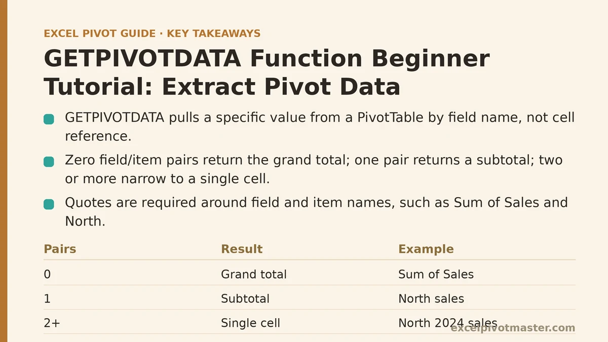
You can supply as few or as many field/item pairs as you need. Zero pairs returns the grand total of that value field. One pair returns a row or column subtotal. Two or more pairs narrow the result to a single cell.
That single rule — more pairs equals a narrower answer — drives every ranked use case below.
Ranked Uses: 5 Ways to Apply GETPIVOTDATA
The list is ordered from most useful for beginners to most advanced, not from easiest to hardest. Rank 1 will solve the majority of real extraction needs; the higher ranks matter once you start building dashboards or line-item reports.
1. Pull a Single Value by Name (The Everyday Use)
What it does: Returns the exact intersection of a value field and one item, using names instead of cell addresses.
Example, with a sales PivotTable having Region in Rows and Sum of Sales in Values:
=GETPIVOTDATA("Sum of Sales", $A$3, "Region", "North")
That formula returns the North region’s sales total. If you later sort the PivotTable, add a new region above North, or move the PivotTable to a different sheet, the formula still returns North’s sales.
Why this ranks first: The cell-reference version of this formula — =B5 — breaks the moment rows shift. If a new region is inserted above North, =B5 now points at the wrong row and there is no error to warn you. GETPIVOTDATA tracks the label, not the coordinates, so it survives layout changes.
When to use it: Any time a formula outside the PivotTable needs one specific figure — a KPI cell, a dashboard tile, a text sentence that quotes a number, or a variance calculation against a prior period.
Typical mistake: Forgetting the quotes around the field and item names. "Sum of Sales" and "North" must be text strings in quotation marks. Writing Sum of Sales without quotes triggers a #NAME? error.
2. Return a Grand Total or a Column Subtotal
What it does: Uses zero or one field/item pair to read a summary rather than a single cell.
Grand total (zero pairs):
=GETPIVOTDATA("Sum of Sales", $A$3)
Returns the overall total of the Sum of Sales field, regardless of filters currently applied to the PivotTable.
Column subtotal with one pair:
=GETPIVOTDATA("Sum of Sales", $A$3, "Region", "North")
Wait — that looks identical to rank 1. It is, when the field called out is also the row field. The distinction matters when your PivotTable uses a page filter or column field. If Year sits in the Columns area, one pair naming a year returns that year’s column total for every row, while two pairs pin down the exact cell.
Practical tip: If you only ever need a single grand-total number, the zero-pair form is the safest formula you can write against a PivotTable. It cannot go stale from a row label change.
3. Chain Pairs to Reach Any Cell in a Cross-Tab
What it does: Adds field/item pairs until the formula describes exactly one cell in a two-dimensional PivotTable.
Example, with Region in Rows and Year in Columns:
=GETPIVOTDATA("Sum of Sales", $A$3, "Region", "North", "Year", 2025)
Note that 2025 is not in quotes. Numeric field items should be passed as numbers, not text. Wrapping a year in quotes often produces a #REF! error because Excel cannot match the text “2025” to the numeric item 2025.
Rule to remember: If the item appears in the PivotTable as a number, pass it unquoted. If it appears as text, pass it quoted. Dates sit in between and are usually safest passed as a date value or text in the exact display format.
Chain limit: You only need as many pairs as the PivotTable has row and column fields. If Region is the only Row field, one "Region" pair is enough regardless of how many columns the layout shows.
4. Read Data From a PivotTable on Another Sheet
What it does: Points the second argument at a PivotTable located on a different worksheet, so a summary tab can reference source figures without opening the data sheet.
Example:
=GETPIVOTDATA("Sum of Sales", 'Sales Pivot'!$A$3, "Region", "North")
The sheet name goes inside single quotes if it contains a space, followed by an exclamation mark before the cell reference — standard Excel syntax.
Why this ranks here rather than higher: Beginners often build a summary tab first and then wire it to a PivotTable on a data tab. The formula works, but it creates a hidden dependency: if someone moves or deletes the PivotTable sheet, the summary tab fills with #REF!. Before wiring cross-sheet references, confirm the PivotTable will stay put.
Safer alternative: Put the PivotTable on the same sheet as the summary figures, or name the PivotTable’s top-left cell with a defined name and reference that name in the formula. A defined name survives sheet renames; a bare sheet reference does not.
5. Generate the Whole Table With a Single Formula Plus Fill
What it does: Uses a locked PivotTable reference and locked field names, with only the item names left unlocked, so one formula can be copied across a grid of rows and columns.
Example, with B$1 holding the row label and $A2 holding the column label:
=GETPIVOTDATA("Sum of Sales", $A$3, "Region", $A2, "Year", B$1)
Fill that across and down, and each cell pulls the matching value from the PivotTable. This is the pattern used for building a summary grid, a mini-dashboard, or a side-by-side comparison that sits next to the PivotTable.
When it pays off: If you need more than about five values extracted from one PivotTable, a fillable grid beats writing five separate formulas. The locking pattern — $A2 for rows, B$1 for columns, $A$3 for the PivotTable anchor, and quotes for the field names — is the whole trick.
When it does not pay off: If the PivotTable layout is likely to change (fields added, removed, or reordered), the field names in the formula become brittle. A #REF! appears the moment a named field disappears.
How Excel Adds GETPIVOTDATA Automatically
When you click a cell inside a PivotTable while writing a formula, Excel usually writes a GETPIVOTDATA formula for you instead of a plain =B5 reference. This surprises people who expect a simple cell reference.
To accept the auto-formula: Just finish typing the formula and press Enter.
To turn the behavior off temporarily: Open the PivotTable Analyze tab, find Options, and clear the “Generate GetPivotData” checkbox. The next cell click produces a normal =B5 reference.
To turn it back on: Same menu, re-check the box.
Which should you use? Keep the auto-generation on. The whole value of the function is that it survives layout shifts, and the auto-generated formula is already correct. Turning it off is only worth doing when you need a fixed cell reference on purpose — for example, when the formula must point at the cell that happens to be in position B5 today and you accept that it will break tomorrow.
Common Errors and What Each One Means
Getting a GETPIVOTDATA formula wrong produces one of four errors. Each one points to a different fix.
- #REF! — The most common. Usually means the field/item pair does not exist in the current PivotTable, or a numeric item was passed in quotes. Check spelling of field names and remove quotes around numeric items like years.
- #NAME? — Almost always a missing or mismatched quote. Every text field and item must be wrapped in straight double quotes (
"), not curly quotes imported from a document. - #VALUE! — Typically a mismatched argument type. Confirm the second argument is a cell inside the PivotTable, not a range that extends outside it.
- #N/A — The request is valid but the item is not present. Confirm the item exists in the current view; a filter hiding the row causes an
#N/Aeven when the underlying data contains it.
Recovery from a corrupted formula: If a formula produces #REF! and you cannot spot the cause, delete the whole formula, click inside the PivotTable, and re-enter it by clicking the target cell. Excel will auto-generate a correct GETPIVOTDATA for you, and you can compare the working version against your broken one.
When NOT to Use GETPIVOTDATA
The function has real limits. Skipping it is the right call in these situations:
- The PivotTable layout is fluid. If fields are likely to be added, removed, or reordered on a regular basis, the formulas become brittle. A
#REF!will appear whenever a named field disappears. - You need to compare against rows the PivotTable filters out. GETPIVOTDATA reads what the PivotTable currently renders; it does not see hidden rows.
- You are pulling a large number of values. Writing thirty GETPIVOTDATA formulas is slower and harder to audit than building a second PivotTable or using
SUMIFSdirectly against the source data. - The data source is structured as a Table. A
SUMIFSformula against the Table name is often faster to write, easier to read, and does not depend on the PivotTable at all.
Rule of thumb: Use GETPIVOTDATA when the PivotTable is the authoritative summary you want to quote, and the layout is stable. Use SUMIFS or INDEX/MATCH against the source when you need flexibility or volume.
Before and After: Plain Reference vs. GETPIVOTDATA
The difference shows up the first time the PivotTable is rearranged. Here is a side-by-side.
| What changes in the PivotTable | Formula using =B5 | Formula using GETPIVOTDATA |
|---|---|---|
| New row inserted above the target | Returns wrong value silently | Returns correct value |
| Rows sorted differently | Returns wrong value silently | Returns correct value |
| PivotTable moved to another sheet | #REF! | #REF! (anchor cell must be updated) |
| Field renamed in the source | Returns blank or wrong value | #REF! — visible failure |
| Row label deleted entirely | Returns wrong value silently | #REF! — visible failure |
The pattern is the same in every row: GETPIVOTDATA either returns the correct value or fails loudly. A plain cell reference tends to fail silently, which is the more dangerous outcome on a report someone else will read.
FAQ-Style Quick Answers
Can I use GETPIVOTDATA on a normal range? No. The function requires a real PivotTable as its second argument. Pointing it at a plain grid produces #REF!.
Does it recalculate when the PivotTable refreshes? Yes. As with any formula, a refresh of the underlying data triggers a recalculation, and GETPIVOTDATA returns the newly refreshed value.
Can it read a value field across multiple value fields? Yes, but only one at a time. If your PivotTable shows Sum of Sales and Count of Orders side by side, you call GETPIVOTDATA twice, once with each data_field name.
What about multiple data fields with the same name? Excel appends a number to distinguish them, such as "Sum of Sales2". Confirm the exact name by clicking the field in the PivotTable’s field list.
What to Do Next
Pick the PivotTable you use most, open a blank cell beside it, and run these three steps in order:
- Click a value cell inside the PivotTable while you have an open formula started. Excel will write the GETPIVOTDATA form for you. Read it back and identify which parts are the
data_field, which is the PivotTable anchor, and which are field/item pairs. - Delete a row from the PivotTable’s source data, refresh, and watch the formula. Note whether the formula returns the new value or an error. That single test tells you whether the formula is tracking labels correctly.
- Copy the formula into a second cell and change only the item name. Confirm the new item returns the correct value without any edit to the anchor or the field name.
Three steps, five minutes, and you will have a working mental model. From there, the ranked list above becomes a reference you come back to when you need a specific pattern — a grand total, a cross-tab cell, or a filled summary grid — rather than something you have to work out from first principles.
Related guides: Excel Pivot Table vs SUMIF: When to Use Which, Power Query Group By Beginner Tutorial: Summarize Data Like Pivot Tables, and Power Query Unpivot Columns: A Beginner Tutorial for Pivot-Ready Data.