A pivot table is the last place most Excel users expect VLOOKUP to work without breaking. The moment you refresh, the row order reshuffles, new categories appear, and old ones vanish — which is exactly why VLOOKUP keeps failing. The counterintuitive part: the fix is not to avoid pivot tables entirely. The fix is to build your lookup against a source that ignores the pivot table’s volatility.
That hidden problem is the grand total row. When you point VLOOKUP at a standard pivot table range, the grand total row sits inside the lookup array. If a key matches the grand total cell, you get a number that is meaningfully different from the category values. Worse, the “Grand Total” label itself breaks exact-match lookups on the first try. You have to exclude that row before you can trust anything.
This guide works through the real questions, in the order they appear when you build a lookup on a pivot table for the first time.
Why can’t I just use VLOOKUP directly on a pivot table?
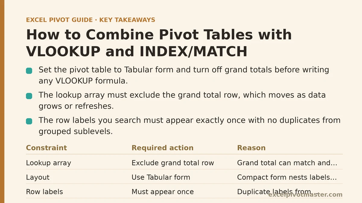
In practice you can, with three constraints. First, the lookup array must exclude the grand total row. Second, the pivot table layout must be in Tabular form — Compact form nests row labels in a way that makes the first column of your range contain merged-looking labels, and VLOOKUP only reads a single column. Third, the row labels you’re searching for must appear exactly once in the pivot table, with no duplicates from grouped sublevels.
Excel will not stop you from pointing VLOOKUP at a Compact layout. It will return values that appear correct for the first few rows, then throw #N/A on every row after a group break. That is not a formula error; it’s a layout mismatch. Switch to Tabular form before writing even one VLOOKUP.
What layout should the pivot table be in before I attempt a lookup?
Set the pivot table to Tabular form and turn off subtotals. Right-click inside the pivot table, go to PivotTable Options, then the Display tab, and uncheck “Show grand totals for rows.” Then go to Design → Report Layout → Show in Tabular Form.
This accomplishes two things. Every row of the pivot table now has identical structure — one category label per row, with no indented sublabels — and the report no longer inserts subtotal rows between groups. Those subtotal rows were creating phantom values in your lookup array that matched nothing but still shifted your row references.
Keep the row field as your single lookup key, and your values field in the column area. A pivot table with two row fields stacked in Tabular form produces duplicate labels for the first field, which breaks any exact-match lookup that expects uniqueness.
How do I exclude the grand total row from my lookup range?
The grand total row appears at the bottom of the pivot table. It is not a static row number — it moves up and down as your data grows, shrinks, or gets refreshed. So you cannot hardcode an absolute range like $A$5:$C$1 as if the pivot table had a fixed shape.
The reliable approach is to define the range dynamically using INDEX. Instead of referencing the whole pivot table output range, build the lookup array to start at the first data row and extend down to the last visible row before the grand total. One formula that does this:
=VLOOKUP($F2, INDEX($A:$B, 1, 1):INDEX($A:$B, MATCH(9.99E+307, $A:$A), 2), 2, FALSE)
The inner MATCH(9.99E+307, $A:$A) finds the last numeric row in column A. Since the grand total row contains a number, you need to adjust: subtract one from that row number. The revised formula excludes the grand total by ending one row above it:
=VLOOKUP($F2, INDEX($A:$B, 1, 1):INDEX($A:$B, MATCH(9.99E+307, $A:$A) - 1, 2), 2, FALSE)
This works because the pivot table’s row labels sit in column A, and after the last data row, the next row is the grand total. The MATCH finds that last numeric row, subtracts one, and your lookup array now covers only genuine data rows.
Why does VLOOKUP return #N/A for some keys even when the key exists?
The most common cause: the pivot table has a filter applied, so that key’s row is hidden. VLOOKUP cannot see hidden rows in a filtered pivot table range. A key that existed in the source data but was filtered out simply is not present in the output range, so VLOOKUP reports it as missing.
The second cause is a blank row label in the pivot table. If any source row has an empty value in the field you’re using as the lookup key, the pivot table groups those rows under “(blank).” That label does not match any key in your lookup list, and the #N/A is correct behavior.
The third cause is case sensitivity. VLOOKUP is case-insensitive, which solves most problems — but if your keys are stored as text in one table and as numbers in another, a mismatch remains. Check for a leading apostrophe or invisible whitespace in your lookup list before suspecting the pivot table.
When should you use INDEX/MATCH instead of VLOOKUP here?
Use INDEX/MATCH when the pivot table has more than two columns and you want the lookup to return a value from a column that appears to the left of the key column. VLOOKUP forces your lookup column to be the leftmost column of the range. In a pivot table, the row labels are always on the left, so that constraint rarely binds — but if your pivot table shows two or three value fields side by side, INDEX/MATCH lets you choose which one to pull without reordering the pivot table.
The second reason to prefer INDEX/MATCH: it handles pivot table column positions after a refresh. When you refresh a pivot table, column headers can shift if new fields appear. VLOOKUP’s third argument (column index number) becomes wrong silently. INDEX/MATCH with a header match rebuilds the column reference each time, so a layout change updates the formula result without manual edits.
A working INDEX/MATCH version for a pivot table, excluding the grand total and referencing the column header in D1:
=INDEX(INDEX($A:$C, 1, 1):INDEX($A:$C, MATCH(9.99E+307, $A:$A) - 1, 3),
       MATCH($F2, INDEX($A:$A, 1):INDEX($A:$A, MATCH(9.99E+307, $A:$A) - 1), 0),
       MATCH(D$1, $A$1:$C$1, 0))
This returns the value where the row label matches F2 and the column header matches D1. The column reference recalculates automatically with each refresh, so header shifts no longer break the formula.
What happens when I refresh the pivot table — will my formulas update correctly?
The formulas above update correctly as long as the pivot table’s row range and column range keep the same starting row. The start row stays fixed at row 1 because the pivot table is anchored there. The end row is dynamic via the MATCH calculation, so new data rows added to the source extend the lookup array automatically.
The one thing that breaks on refresh is the column header reference in INDEX/MATCH. If you have a header that says “Sum of Revenue” and a refresh collapses two old columns and adds a new one, the header text stays static. The formula still finds the correct column by matching that header, so no manual fix is needed.
If you change the field being summarized in the Values area — say from Revenue to Count of Orders — the header text changes, and your INDEX/MATCH formula returns the wrong column. Update the header cell in your formula to match the new header text.
There’s a smarter approach for large or frequently refreshed data — what is it?
Build the lookup against the source data table, not the pivot table. Every pivot table is a summary of a larger flat table. VLOOKUP works cleanly on that source table because it has no grand total row, no subtotal rows, and no layout transformations.
This approach has one caveat: the source table lacks the pivoted structure. If your pivot table shows categories in rows and months in columns, the source table has months in rows, not columns. You would need a pivot table to reshape it. So the real question is whether you need a wide, pivoted shape — in which case the pivot table is the right output — or a narrow matching problem where the source table suffices.
A hybrid approach handles both concerns: keep the pivot table as your report, then add a lookup column beside the pivot table that pulls from the source table using SUMIFS. This avoids the pivot table entirely for calculation purposes and keeps your formulas stable regardless of pivot layout. The pivot table becomes a display layer; the formulas work against a clean, structured input.
How do I stop my formulas from breaking when someone changes the pivot table layout?
Set the pivot table range as a named range that references the last row dynamically, and build all formulas against that named range. Excel’s pivot table output range is volatile, but a named range built with OFFSET and COUNTA captures the live shape.
Define a named range called PivotData as:
=OFFSET($A$1, 0, 0, COUNTA($A:$A) - 1, 3)
This skips the grand total row automatically, since COUNTA($A:$A) - 1 counts all rows in column A and subtracts one for the total. Now VLOOKUP and INDEX/MATCH formulas reference PivotData instead of hardcoded ranges. If the person on your team converts the pivot table to Compact form, the named range still covers the same cells — but the layout change itself will still break the lookup due to the nested label issue. The named range protects against row count changes, not layout changes.
For layout protection, the only reliable defense is to keep the pivot table in Tabular form and communicate that constraint to anyone who might change it.
Quick Reference for Pivot Table Lookups
| Symptom | Likely Cause | Fix |
|---|---|---|
#N/A on keys that exist | Filter in the pivot table hides the row | Clear filters or use SUMIFS on source data |
| Wrong value returned in the grand total row | Grand total row inside the lookup array | Dynamic range that excludes the last row |
| Lookup fails after refresh | Pivot table row order changed but range is static | Use OFFSET-based named range or dynamic INDEX/MATCH |
#N/A on all rows after first group | Compact layout nests labels | Switch to Tabular form |
| Wrong column returned | Column index hardcoded after header shift | Use INDEX/MATCH with header match |
The pivot table was never designed as a lookup source. It is a reporting tool that has a changing shape — that is why raw VLOOKUP fails. In practice, the dependable combination is: Tabular form, no grand total, and a dynamic range built with INDEX or OFFSET. With that structure in place, you get a lookup that behaves like a static table but adapts to every refresh.
Once that version works, consider whether you need the pivot table in the formula at all. If the answer is no, SUMIFS on the source table gives you a faster, cleaner, and layout-independent result. The pivot table stays for reports; the formulas stay for math.
Related guides: Using GETPIVOTDATA to Build Dynamic Reports from Pivot Tables: Beginner Tutorial, Excel Pivot Table vs SUMIF: When to Use Which, and GETPIVOTDATA Function Beginner Tutorial: Extract Pivot Data.