A range that spans one worksheet and a range that spans several worksheets look almost identical when you select them. That resemblance is the trap. Selecting Sheet1!A1:D50 gives a pivot table one flat block of data to read. Selecting Sheet1!A1:D50 and Sheet2!A1:D50 as two separate areas does not automatically merge them into one dataset — it asks Excel to treat them as a single source, which it can only do if the columns line up perfectly, and which produces very different results depending on whether you route through Power Query, the Data Model, or the legacy Consolidate dialog. Beginners pick the wrong path and then spend an afternoon wondering why their row labels are blank.
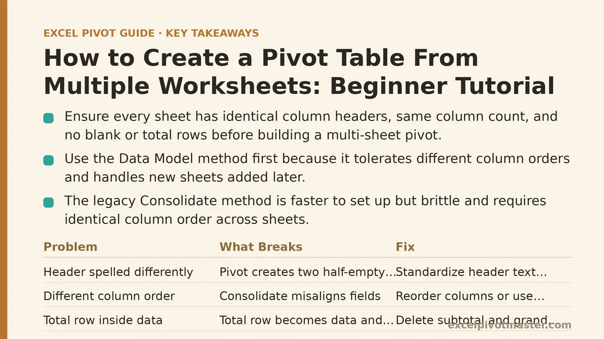
This tutorial walks through the two reliable methods for building a multi-sheet pivot table, in the order most beginners should attempt them. Both take under fifteen minutes once the source data is clean. The first method (the Data Model) is the one to learn first because it handles mismatched column order and handles new sheets added later. The second (the legacy Consolidate range) is faster to set up but brittle, and it is worth knowing so you can recognize it when a downloaded template uses it.
Before any of that, the data has to pass a preparation check. Skip that check and both methods fail in ways that look like Excel bugs.
Before You Start: The Three Rules Your Source Sheets Must Follow
Multi-sheet pivots fail for structural reasons, not formula reasons. Confirm all three of these before opening the PivotTable wizard.
Rule 1 — Every sheet has the same column headers, spelled identically. “Region” and “region” and “Region " (with a trailing space) are three different fields to Excel. The pivot will create three separate columns, each half-empty.
Rule 2 — Every sheet has the same number of columns, in the same order if you are using the Consolidate method. The Data Model tolerates different column orders; the Consolidate range does not. If your sheets are Jan-Sales, Feb-Sales, Mar-Sales and Jan has an extra “Notes” column at the end, remove it or the header row before combining.
Rule 3 — No blank rows and no total rows inside the data. A “Total” row halfway down a sheet becomes a normal data row in the consolidated output and inflates every sum downstream. Delete subtotal and total rows before the pivot is built, not after.
Run through this checklist on each sheet once. It takes two minutes and prevents most of what follows.
| Problem in the source sheets | What breaks | Fix before building |
|---|---|---|
| Header spelled differently on one sheet | Pivot creates two columns, each half-empty | Standardize the header text exactly, no extra spaces |
| Different column order across sheets | Consolidate misaligns fields; totals look wrong | Reorder columns or use the Data Model method instead |
| A total row inside the data block | Total row becomes a data row and doubles sums | Delete subtotal and grand total rows first |
| Blank row between data blocks | Rows after the blank are dropped | Fill or delete blank rows so data is contiguous |
| A sheet named “Sheet1” with a space in front | Range reference fails silently | Rename sheets to simple names before referencing |
Step 1: Decide Which Method Fits Your Sheets
Two methods produce a working multi-sheet pivot. They differ in what they demand from your source data.
The Data Model method builds a single table from your sheets using Power Query or the internal Data Model. It is the modern approach, handles column order differences, and automatically includes new sheets you add to the same workbook later if you use Power Query’s folder or table-append approach. Higher learning curve, more robust result.
The Consolidate range method uses the older “Multiple Consolidation Ranges” option in the PivotTable wizard. Every sheet must have an identical layout. Setup takes about three minutes. If you add a fourth sheet next quarter, you have to rebuild.
For a one-off monthly report where the sheets are already identical, use Consolidate. For anything you will run more than twice, use the Data Model. The rest of this tutorial covers both, starting with the one you should learn first.
Step 2: Open the PivotTable Wizard’s Multi-Range Option (Consolidate Method)
This method requires a keyboard shortcut because the multi-range option is not on the ribbon.
- Select any cell in an empty area of a fresh worksheet — a new sheet is best so the output is not tangled with source data.
- Press Alt, then D, then P in sequence (not held together). A small PivotTable and PivotChart Wizard dialog opens.
- Choose Multiple consolidation ranges, then Next.
- Choose I will create the page fields, then Next.
The “page fields” option creates one filter field that lets you switch between the source sheets in the resulting pivot. If you skip it and choose “Create a single page field for me,” Excel generates a page field automatically and the resulting layout is harder to filter.
Step 3: Add Each Worksheet’s Range (Consolidate Method)
The dialog now asks you to list each range. Click in the Range box, then click over to the first sheet and select the data including the header row.
- Type or select the range for sheet 1 — for example,
Jan!$A$1:$D$51. - Click Add. The range moves into the “All ranges” list.
- Repeat for each remaining sheet: select the range, click Add.
- When every sheet is listed, click Next.
Critical constraint: All ranges must have the same number of columns, and the column order must match. If Jan has Date, Region, Product, Units and Feb has Date, Product, Region, Units, the consolidated pivot will treat Product in Jan as a different category than Product in Feb. It will not throw an error. It will just produce wrong totals.
Choose where the new pivot goes — a new worksheet is safer — then click Finish.
The pivot appears with generic field names: Row, Column, Value, and Page1. These correspond to the first column, second column, third column, and the page field that identifies the source sheet. Rename them mentally: Row is your first source column, Column is your second, Value is your numeric column, Page1 is the sheet name.
Drag Value into the Values area. Drag one or two of the others into Rows or Columns. The totals now span every sheet.
Step 4: Build the Data Model Version (The Method to Use for Recurring Reports)
The Data Model approach produces a cleaner result and does not require identical column order across sheets. It uses Power Query, which Excel has shipped as a built-in feature since 2016.
- First, convert each source sheet into a formatted Excel Table. Select the data, press Ctrl+T, confirm the header row, and give the table a clear name in the Table Design ribbon —
JanData,FebData,MarData. - On each subsequent sheet, repeat: Ctrl+T, name the table.
- Go to the Data ribbon → Get & Transform Data → Get Data → From Other Sources → Blank Query (or, on newer builds, use Data → From Table/Range and append each named table in sequence).
- In the Power Query editor, use Home → Append Queries → Append Queries as New. Add each of your named tables in the order they appear. Power Query matches columns by name, so different column order across sheets is fine.
- Check the column headers at the top of the resulting table. Rename any that Power Query auto-suffixed (e.g., “Product.1” means a mismatch it could not resolve).
- Click Close & Load To… and choose PivotTable Report as the destination. This loads the appended data into the Data Model and creates a pivot on a new sheet in one step.
The resulting pivot has real field names — Date, Region, Product, Units — not Row/Column/Value. That alone is worth the extra four minutes of setup. Adding a new sheet next quarter means appending one more query step, not rebuilding the pivot from scratch.
Step 5: Add a Source Identifier Column (Optional but Strongly Recommended)
Neither method tells you, at the row level, which sheet a number originally came from — unless you add a helper column first.
Before building the pivot, add a column called Source to every sheet and fill it with the sheet name or month (“Jan”, “Feb”, “Mar”). Then include that column in your selection or your Table range.
Now you can drag Source into the Rows or Columns area and see, for example, January sales in one column and February sales beside it. Without this column, a multi-sheet pivot gives you consolidated totals with no way to break them back apart by origin. Adding it takes thirty seconds per sheet.
This is also the step that catches the “which sheet is this row from” question before the report is shared with anyone.
Step 6: Verify the Result Against the Source Totals
A multi-sheet pivot that looks right can still be wrong. Confirm it before using it.
- Sum the numeric column on each source sheet with
SUM(). Add the three or four totals in your head or on a scratch cell. - Compare against the pivot’s grand total.
- If they match to the cent or the unit, the pivot read every range it was asked to.
- If they differ, the most likely cause is a sheet that was not added to the consolidation list, or a range that missed the last few rows.
Do this check once, every time the pivot is rebuilt. It takes ninety seconds and catches the majority of silent errors. A pivot that undercounts by one missing sheet looks exactly like a pivot that is correct.
Common Mistakes and How to Recover
Mistake: Column headers differ by capitalization or spacing across sheets. Recovery: Standardize headers on every sheet with Find & Replace, then rebuild the pivot. Changing headers on the source sheets after the pivot is built does not update the pivot’s fields — you must rebuild or edit the Data Model query.
Mistake: Using the Consolidate method and later adding a fourth sheet. Recovery: You cannot add a range to an existing Consolidate pivot. Rebuild it. This is the reason to prefer the Data Model for anything recurring.
Mistake: Selecting whole columns (A:D) instead of the data range. Recovery: Whole-column references in the Consolidate dialog pull in blank rows and inflate row counts. Go back through the wizard and set exact ranges, or convert to Tables first.
Mistake: Blank row in the middle of one sheet’s data. Recovery: Find and delete the blank row on the source sheet, then refresh. In the Consolidate method, the pivot silently drops rows after the blank — it does not warn.
Mistake: One sheet has a “Total” row at the bottom included in the selection. Recovery: Exclude the total row from the range. If it was included, delete the phantom row from the pivot output or rebuild with a corrected range. Leaving it in will double your grand total.
Mistake: The pivot created fields named “Row”, “Column”, “Value”, “Page1” and the labels are meaningless. Recovery: You used the Consolidate method. The field names come from the wizard, not your headers. Rename them in the pivot field list (PivotTable Analyze → Field List → double-click a field name) or switch to the Data Model method for readable field names.
Before and After: What a Correct Multi-Sheet Pivot Looks Like
| Check | Wrong result | Correct result |
|---|---|---|
| Grand total vs. sum of each sheet’s totals | Under-counts by one sheet | Matches exactly |
| Row labels | Generic “Row”, “Column”, “Value” (Consolidate method) | Real field names from your headers (Data Model) |
| Adding a sheet next quarter | Rebuild the whole pivot (Consolidate) | Append one power query step (Data Model) |
| Column order differences across sheets | Silently misaligned totals (Consolidate) | Handled automatically (Data Model) |
| Source tracking | Cannot tell which sheet a number came from | “Source” column lets you split by sheet |
If any row on the left matches what you are currently seeing, the recovery step is either to swap to the Data Model method or to go back and fix the source sheets.
What to Do Next
Pick the workbook you most often combine across sheets — monthly sales, quarterly expenses, weekly time logs — and do this today:
- Confirm the three source rules on each sheet: identical headers, same column count, no total rows inside the data.
- Add a “Source” helper column to each sheet with the sheet name or period label.
- Convert each sheet to a Table (Ctrl+T) and give it a name.
- Build the pivot using the Data Model method (Get Data → Append Queries → Close & Load To → PivotTable Report).
- Verify the grand total against a manual sum of the individual sheet totals.
Once this runs cleanly on one workbook, the same five steps apply to any multi-sheet dataset. The Consolidate method still works for one-off reports where the sheets are already identical, but the Data Model version is the one that survives a fourth sheet being added next quarter without being rebuilt from scratch.
Related guides: Pivot Table Not Refreshing: Common Causes and Fixes, Fixing Pivot Table Refresh Errors and Stale Data Problems, and Pivot Table Not Showing All Data: Fix Guide for Every Cause.