Dragging a date field into the Rows area gives you a pivot table with one row per date. Right-clicking that field and choosing Group gives you a pivot table with one row per month. Those are two different operations that people routinely treat as the same thing, and the confusion between them sits behind most of the failed grouping attempts you will run into.
The first is a display choice. The second rebuilds how the pivot cache stores the field — it creates a grouped date hierarchy that Excel can roll up into quarters and years. If you expect the right-click menu to behave like the first and it behaves like the second, or the other way around, the result looks wrong for reasons that have nothing to do with your source data. What follows separates the myths from what is really happening, then walks through the fixes that hold.
Myth: Any column that looks like a date can be grouped
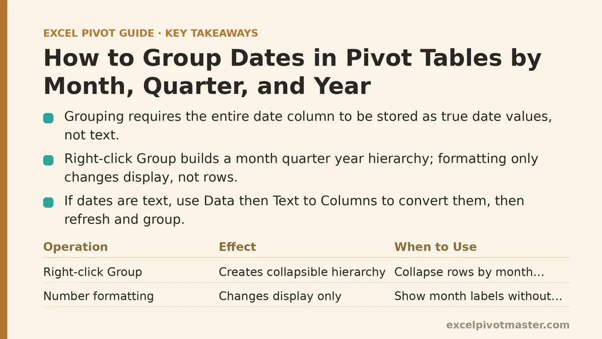
Reality: Grouping requires the entire column to be stored as true date values.
This is the first wall most people hit, and the error message does not name it directly. Right-click a date field, choose Group, and Excel reports that it “cannot group that selection” or that the selection “cannot be grouped.” The instinct is to assume the pivot table is broken. The column is almost always the problem.
A column of dates that were pasted from another system, exported from a report, or typed with inconsistent separators commonly arrives in Excel as text, not as dates. Text that reads “01/15/2026” is a string of characters that happens to look like a calendar date. Excel stores it that way and offers no grouping options for it, because there is nothing to roll up — the field has no underlying year, month, or day values to extract.
The check: Select the date column in your source data and look at the alignment. True dates right-align by default. Text dates left-align. If the column leans left, that is your cause.
The fix: Select the whole column, go to Data → Text to Columns, keep the default delimited settings, and finish the wizard. This forces Excel to reinterpret each cell, and a column of recognizable date text is converted to real date serial numbers. Refresh the pivot table and try grouping again. For a column where the values are ambiguous — some cells “3/4/2026” with no clear month-day convention — set the column format to Date explicitly before running the wizard so Excel interprets consistently.
Myth: Right-click Group is the same as the field’s date format settings
Reality: Grouping builds a hierarchy; formatting changes how individual values display.
Two controls sit near each other and get mixed up constantly. The first is the right-click Group command on a date field in the Rows area. The second is the value field settings under PivotTable Analyze → Field Settings → Number Format, or the “Show values as” options in the Values area.
Only the first one creates month, quarter, and year groupings. The second one can make a full date display as “Jan” while the underlying field remains a separate item per day. You can format a date field so the cells read “January 2026” and still have 47 rows in the pivot table, one for each day in that month, because formatting never merges rows.
If you want rows collapsed by month: use right-click Group. If you want each day’s row to display a month label without collapsing: use formatting alone. Choosing the wrong one is the reason a pivot table can look grouped while behaving like it is not.
Myth: Grouping by month is the only useful option
Reality: Excel exposes one dialog that produces month, quarter, and year in a single grouping step.
When you right-click a date field and choose Group, the Grouping dialog opens with two boxes labeled Starting at and Ending at, pre-filled with the earliest and latest dates in your field. Below them sits a list of checkboxes: Years, Quarters, Months, and sometimes Days. Checking two or more of these builds a nested hierarchy in one pass.
Three combinations cover most reporting work:
- Months only — one row per month across all years present, useful for seasonal comparisons where year does not matter.
- Years + Months — a year row for each year, with months nested underneath, which is the standard layout for multi-year reporting.
- Years + Quarters + Months — a full calendar hierarchy, useful when a quarterly view and a monthly view are both needed from one table.
If you select Years and Months together and click OK, the Rows area shows a year item with a collapse arrow, and expanding it reveals the twelve month items beneath. There is no need to build three separate pivot tables to get three levels of detail.
Myth: Grouping by quarter means typing a quarter formula in the source data
Reality: Excel derives quarters from the grouped date field with no helper column required.
A common workaround is to add a =ROUNDUP(MONTH(A2)/3,0) column to the source data so the pivot table can summarize by quarter. That works, and for some edge cases it is the right approach, but it is not necessary for ordinary quarter reporting.
Check the Quarters box in the Grouping dialog and Excel adds a Quarter field to the same hierarchy. Each quarter shows as Q1, Q2, Q3, or Q4, and the year sits above it when Years is also checked. The pivot table rolls the underlying daily or monthly values into the quarters automatically.
When the helper column is still warranted: if your fiscal year does not begin in January, Excel’s default quarter grouping uses calendar quarters, and a Q1 label will not match a fiscal Q1 that starts in April. In that case a =CHOOSE(MONTH(A2),4,4,4,1,1,1,2,2,2,3,3,3) style column, or the equivalent =ROUNDUP((MONTH(A2)+9)/3,0) adjusted for the fiscal start, gives you the fiscal quarter. Group on that column instead of the raw date.
Myth: Once grouped, the field stays grouped through every refresh
Reality: Grouping is stored in the pivot cache and can drop or misbehave when the source data shifts.
Grouping is not a per-session setting. It is written into the pivot cache when you apply it, and it normally survives refreshes. Where it breaks is when the source range changes shape in ways that interact badly with cache settings.
Two situations cause this:
- New dates before the grouped starting point. If you grouped with Starting at 2025-01-01 and later add a January 2024 record to the source, the grouping does not automatically extend backward. The new date may appear as an ungrouped row above the year rows, or be silently excluded depending on the cache’s item retention setting.
- Number of items to retain per field set to Automatic. This cache setting, found under PivotTable Options → Data, keeps old field items so filters and layouts stay stable. It also means grouped items can linger with stale labels after source changes. Setting this to None on any pivot table whose data gets rows added or deleted removes that risk.
The fix when grouping drops after a refresh: Right-click the date field → Ungroup, then reapply Group with the range extended to cover the new earliest and latest dates. If you add data routinely, extend the Ending at box a year or two past today’s last date so the grouping has headroom.
Myth: Every date field in the Rows area can be grouped the same way
Reality: Grouping only applies to one date field at a time, and mixing date fields causes errors.
Excel permits exactly one grouping per pivot table based on a single date field. If you drag two separate date columns into the Rows area — say an Order Date and a Ship Date — and try to group both, the second attempt throws an error because adding a second grouped date field creates a hierarchy Excel cannot reconcile.
The typical symptom is a message about the field already being grouped, or a group dialog that refuses to open. The cause is the existing group on the first field, not the second field’s contents.
The recovery path: Ungroup the first field (right-click → Ungroup), decide which date field you need at the top of the hierarchy, group that one, then use the second date column as a Values field, a column label, or a filter instead of a row field. For side-by-side date comparison, build two pivot tables sharing the same cache — one grouped on Order Date, one grouped on Ship Date — and place them next to each other.
Myth: Grouping a date field in one pivot table groups it everywhere
Reality: Grouping belongs to the cache, so shared-cache tables follow and separate-cache tables do not.
Pivot tables built by copying an existing pivot table, or by pointing multiple tables at the same source range through the wizard, typically share one cache. Group the date field once and the grouping appears in each table that shares it. Pivot tables built independently have separate caches and their own grouping state.
This is why you can group a date in one table and see ungrouped dates in the table next to it. It has the same feel as the shared-versus-separate cache behavior that affects refresh. The fix, if you want them aligned, is to delete the independently-built tables and rebuild them by copying the grouped table and re-pointing it at the source, so they share the cache.
Myth: Grouping a field order like Q1 2025, Q2 2025 sorts correctly by default
Reality: Sort order follows the underlying date value, not the label text, unless you override it.
Grouped fields sort chronologically by default, which is usually what you want. The misfires happen when a custom sort was applied before grouping, or when the group labels are being treated as text because the underlying value is text masquerading as a date.
If quarters appear as Q1, Q10, Q2 — an ordering impossible in a calendar year but common in text sorting — the group labels are sorting as strings. The root cause is usually that the underlying field was text and grouping silently failed, leaving Excel to display the raw text values in a nonsensical order. Going back to the source column, running Text to Columns, and reapplying grouping restores the chronological sort.
For a fiscal-year view where you want Q4 of the last fiscal year to sit before Q1 of the next, group on a fiscal quarter index column rather than the raw date, so the sort key matches the reporting period.
Myth: The “Group” option is always in the right-click menu
Reality: The menu item appears conditionally, and its absence is itself a diagnostic.
Right-click a date field in the Rows or Columns area and the menu should include Group. If it does not appear:
- The field is not being treated as a date. Confirm the source column is stored as date values.
- You are right-clicking a value cell rather than the field label. Click the field header first, or right-click the cell and select Group from the resulting menu carefully.
- The pivot table contains no date field. Grouping is available only for date and numeric fields.
- A hidden or filtered date item is blocking the group. Clear all filters on the date field and try again.
The presence or absence of the Group item is a quick test of whether Excel recognizes the field as a date, and it costs nothing to check before you start editing source data.
Before and After: What a Correct Date Grouping Produces
| Situation | Ungrouped field | Correctly grouped field |
|---|---|---|
| Row label for January 2026 | One row per day | One row labeled “Jan” (or “Q1” if grouped to quarter) |
| Fiscal-year reporting | Calendar quarters, misaligned to fiscal periods | Fiscal quarters, aligned to your year start |
| Multi-year data | Long list of individual dates | Collapsible Years → Quarters → Months hierarchy |
| Added records after grouping | Silently excluded or shown ungrouped | Included when the group range has headroom |
| Second date field in Rows area | Both can sit side by side | One must be ungrouped or moved out of the row area |
| Two pivot tables on the same range | Grouping may differ between them | Same grouping if they share a cache |
The right-hand column is what you should see once a date field is grouped correctly. Where the left column describes your table, work the corresponding myth above.
What to Do Next
Open a workbook with a pivot table built on a date column, and run these checks in order today:
- Confirm the date column is stored as dates. Select it in the source data and check the alignment. Right-aligned means true dates; left-aligned means text. Run Text to Columns if it is text.
- Apply the group you need. Right-click the date field in the Rows area → Group → check Months, Quarters, and Years as required. Widen the Starting at and Ending at boxes to cover at least a year of future data.
- Set item retention to None. PivotTable Options → Data → “Number of items to retain per field” → None, if this table gets rows added or deleted over time.
- Refresh and confirm the hierarchy collapses correctly. Expand a year and check that the quarter and month children appear in calendar order, not string order.
Those four steps cover the situations that account for the large majority of date grouping failures — text dates, narrow group ranges, and cache item retention. If a problem persists after all four, note which step in the myth list matches what you are seeing and what Excel’s error message said word for word; that combination narrows the cause faster than rechecking settings you have already ruled out.
Related guides: Excel Pivot Table: Group Dates by Month and Year (Without the Headaches), Data Model Relationship Errors in Excel Pivot Tables: 7 Common Failures and How to Troubleshoot Them, and How to Remove Blanks from Excel Pivot Tables: Every Cause and Fix.