A large dataset, for the purpose of this guide, is anything that makes Excel start feeling sluggish when you open the file, drag a field into the Row area, or hit Refresh. In practice, that threshold lands somewhere between 50,000 and 200,000 rows depending on your hardware, the number of columns, and whether you are using the 32-bit or 64-bit version of Excel. Above that range, slowness becomes the default state, and that slowness is not random — it traces back to specific, addressable causes.
Step 1: Turn Your Source Data Into a Proper Excel Table
Before a pivot table ever touches your data, the source range itself deserves attention. A raw range of cells — say, A1:Z180000 — works, but it creates problems that compound as the data grows.
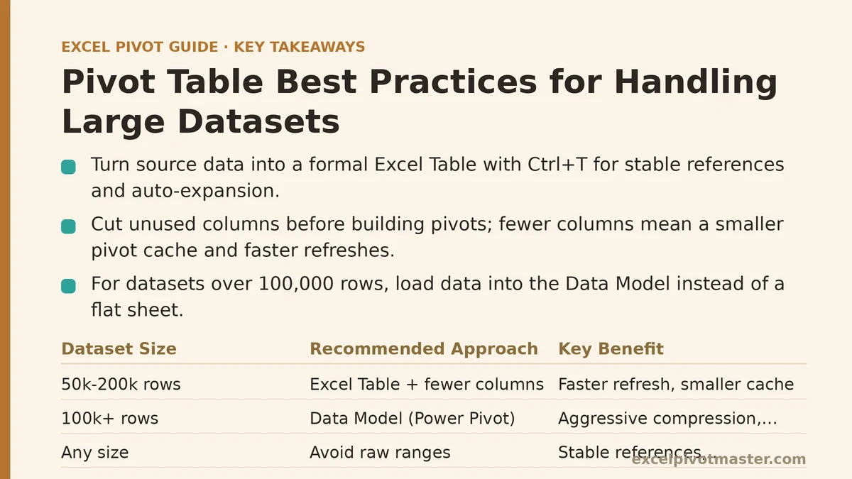
Select any cell inside your data, press Ctrl+T, and confirm the Create Table dialog. This single step converts the range into a formal Excel Table, which brings three performance-relevant benefits. First, the table has a defined name (Table1, Table2, and so on) that you can reference directly in the pivot table’s source field, so the pivot cache points at a stable, named object rather than a fragile range. Second, any new rows appended to the bottom of the table automatically extend the table’s bounds, which means your pivot table picks up new data on refresh without you manually resizing the source range. Third, Excel’s internal handling of structured references is more efficient than its handling of raw cell ranges, which shows up as faster calculations when the pivot table refreshes.
If you are using Power Pivot or the Data Model — which Step 3 will cover in detail — the Excel Table also serves as the cleanest possible ingestion point, since Power Pivot is designed to consume named tables directly.
Step 2: Cut the Columns Down Before Building the Pivot
Every column you carry into a pivot table adds overhead at refresh time, and a surprising amount of that overhead comes from columns you never use. A 200,000-row dataset with 60 columns contains 12 million cells total. If your pivot table only uses 8 of those columns, the other 52 are still being loaded into the pivot cache on every refresh, eating memory and slowing the process.
Before you build the pivot table, scan the dataset for columns that serve no analytical purpose — notes fields, internal IDs, merged helper columns, raw timestamps that you will only ever group by month anyway. Delete them from the source, or at minimum, select only the columns you need when you create the pivot table. In the Create PivotTable dialog, this is easy: instead of selecting the entire table, select just the columns you plan to use, give that selection a name (for example, PivotSource), and point the pivot table at that named range.
This approach is not about being precious about disk space — it’s about refresh speed. Fewer columns means a smaller pivot cache, which means faster refresh cycles and less memory pressure when Excel recalculates.
Step 3: Use the Data Model Instead of a Flat Sheet
Once your dataset crosses into the 100,000-plus row territory, the smartest structural decision you can make is to stop pointing your pivot table at flattened worksheet data entirely. Instead, load the data into the Data Model — Excel’s in-memory columnar database that sits behind Power Pivot — and build your pivot table from there.
The Data Model compresses data aggressively. A flat worksheet with 300,000 rows of repetitive text — customer names, product categories, region labels — can shrink to a fraction of its original size when loaded into the Data Model, since the columnar storage deduplicates repeated values automatically. Pivot tables built on the Data Model refresh noticeably faster on large datasets, and they open the door to DAX measures, which let you calculate things like running totals and year-over-year comparisons without the helper-column headaches covered in earlier guides on running totals.
Setting this up is straightforward: in the Create PivotTable dialog, check the box labeled “Add this data to the Data Model.” If you have already loaded the data via Power Query (Get & Transform Data → From Table/Range), you can create the connection to the Data Model from the Power Query editor itself by closing and loading the query with the “Only Create Connection” option selected, then building your pivot from that connection.
One trade-off is worth naming plainly: the Data Model has a hard 2 GB memory limit, and while that sounds generous, it counts compressed data, not raw rows. In practice, you can get hundreds of thousands of rows into the Data Model without issue, but if you are working with millions of rows, your bottleneck will be available RAM in your machine, not Excel’s limits.
Step 4: Control the Pivot Cache’s Item Retention
The pivot cache — the hidden in-memory snapshot of your source data that the pivot table reads from — maintains a list of every distinct item it has ever seen for each field, even after you delete rows from the source data. This is the same mechanism that causes stale entries to linger in filter dropdowns, covered in the post on removing blanks, but for large datasets it has a more serious consequence: the cache grows a little larger every time the source data changes, and over many refreshes, that growth becomes measurable.
Fix this in PivotTable Options. Right-click the pivot table, choose PivotTable Options, go to the Data tab, and change “Number of items to retain per field” from Automatic to None. This tells Excel not to keep historical item lists hanging around after refresh. With this setting applied, a pivot table built from volatile source data — where rows are added and removed frequently — will keep its cache lean, refresh faster, and avoid the slow creep of stale items.
If you are already using the Data Model from Step 3, this setting no longer applies directly, since the Data Model is a database rather than a per-pivot cache. But if you are working with classic pivot tables against worksheet ranges, this is one of the highest-leverage speed tweaks available.
Step 5: Aggressively Reduce What’s Displayed in the Report Itself
A large dataset does not have to become a large pivot table on screen. If your report is being shared with decision-makers, or if you are the one staring at it all day, a pivot table that expands to 80,000 rows of line items is not useful — it is a wall of noise.
Set the pivot table to Group by Date, by Quarter, or by Year if your data has a date field. Grouping is the single fastest way to collapse thousands of transaction-level rows into a few dozen summary rows. For text fields, drag a field like Region or Category into the Row area instead of Customer Name or Transaction ID. This shifts the grain of the report from granular to summary, and the pivot table’s performance improves automatically because there are simply fewer rows to render.
Also use the filter area deliberately. A Slicer or a report filter that limits the pivot table to a single region or timeframe reduces the visible result set to a small fraction of the full data, and the pivot table recalculated from that filtered subset renders far more quickly than one spanning everything.
Step 6: Turn Off Automatic Refresh and Recalculate While Editing
By default, Excel recalculates the entire workbook whenever any cell changes. With a huge dataset sitting behind a pivot table, that recalculation — combined with the pivot table’s auto-refresh behavior — can make every small edit to the workbook a multi-second pause.
Open the PivotTable Options, go to the Data tab, and uncheck “Refresh data when opening the file.” This stops the pivot from force-refreshing every time you open the workbook, which matters for large files that take several seconds to refresh on load. You will still need to refresh manually (right-click → Refresh) when you want the latest data, so make that a deliberate step.
Also consider switching the workbook to Manual Calculation mode while you are actively editing formulas elsewhere. Go to Formulas → Calculation Options → Manual, edit whatever you need, and press F9 to recalculate manually when you are done. This does not affect the pivot table’s own refresh (pivot tables have their own refresh mechanism separate from Excel’s calc engine), but it does stop the whole workbook’s formula engine from grinding through 200,000 rows’ worth of dependencies on every keystroke.
Step 7: Measure the Before-and-After
The final step is verification. When you apply any of these changes, measure the impact rather than assuming it worked.
Time a full refresh cycle before you make changes — right-click the pivot table, hit Refresh, and time how many seconds pass before the status bar stops showing progress. Repeat after each change. A pivot table that took 25 seconds to refresh and now takes 8 seconds, or a workbook that opens in 4.5 seconds instead of 15, gives you concrete evidence that a given practice is worth keeping.
Similarly, watch the taskbar’s memory usage in Task Manager while the pivot table refreshes. If you consistently see Excel consuming 800 MB or more while working with your data, the Data Model path in Step 3 becomes less of a nice-to-have and more of a necessity.
Quick Reference: Where to Look When Things Still Feel Slow
| Symptom | Likely Cause | Best Practice That Fixes It |
|---|---|---|
| Refresh takes multiple seconds | Large cache from an ungroomed source range | Convert to Excel Table, use Data Model, set item retention to None |
| Workbook opens slowly | Auto-refresh on file open | Turn off “Refresh data when opening the file” |
| Editing any cell stalls | Formula engine recalculating everything | Switch to Manual Calculation while editing |
| Pivot table renders thousands of rows | No grouping or filtering applied | Group by date, filter by region/timeframe |
| Memory peaks above 800 MB | Flat worksheet data being loaded into classic pivot cache | Move source into the Data Model |
| Stale items linger in dropdowns after row deletions | Pivot cache retaining old item lists | Set “Number of items to retain per field” to None |
Each of these steps works independently, but they compound when used together. A properly structured Excel Table feeding a Data Model pivot with grouping, filters, and a lean cache will handle datasets that would otherwise grind a classic pivot table to a halt. The order above arranges the changes roughly by impact, from structural foundation at the start to everyday habits at the end.
The distinction between a large dataset and a slow workbook is rarely unavoidable — it is almost always a design choice. Make it early, and the rest of your work with that data becomes consistently faster.
Related guides: 5 Pivot Table Setups Every HR Analyst Needs for Headcount and Attrition, Excel Pivot Table Common Errors and Fixes: A Real Troubleshooting Walkthrough, and Excel Pivot Table Layout Styles: Compact vs Outline vs Tabular Explained.