A pivot table that throws “Reference is not valid” and a pivot table that throws “PivotTable field name is not valid” sound like twins, but they are unrelated. The first points to the data range the pivot table draws from; the second points to a header inside that range. Blend the two, and you will spend time renaming columns that were never the problem.
This guide follows a checklist format. Start at Step 1. Each step either fixes the error or eliminates a cause so you can move to the next one without repeating work.
Step 1: Is the Error About the Range or the Field Names?
When the message appears, read it in full before clicking anything. The two most common variants are:
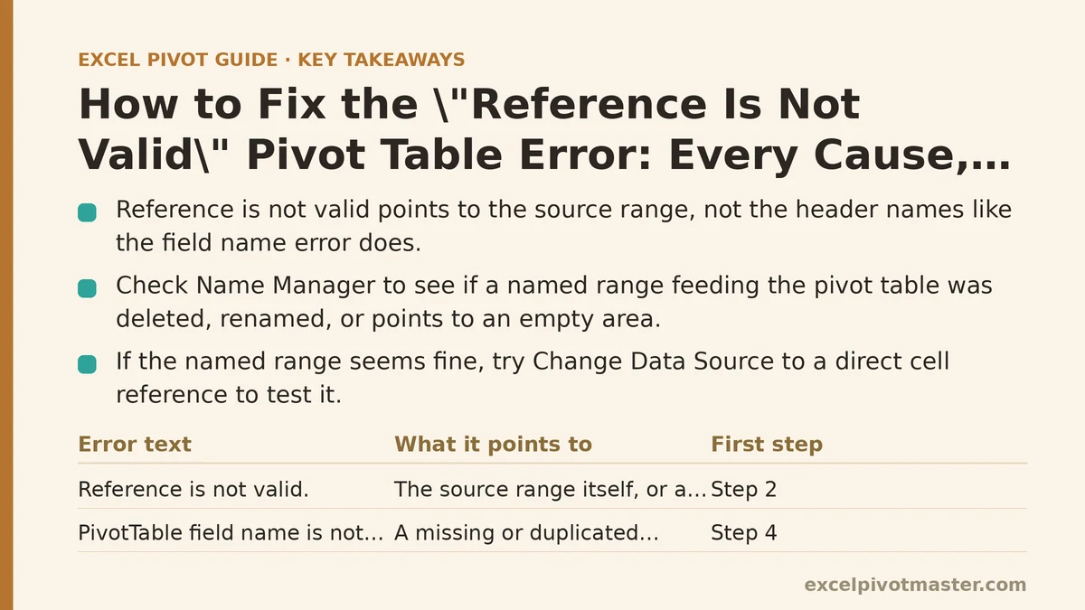
| Exact error text | What it points to |
|---|---|
| “Reference is not valid.” | The source range itself, or a named range feeding the pivot table |
| “PivotTable field name is not valid.” | A missing or duplicated header row inside the source range |
If your message includes the “field name” phrase, skip to Step 4. If it says only “Reference is not valid,” continue here.
Step 2: Check Whether the Named Range Still Exists
If your pivot table draws from a named range — for example, you typed SalesData into the Table/Range box instead of Sheet1!$A$1:$F$500 — the error often appears because that name was deleted, renamed, or now points to a range that no longer exists.
Open the Formulas tab and click Name Manager. Look for the name your pivot table references. If the name is missing, your pivot table’s source has nothing to point at. Recreate the name, or switch the pivot table to a direct cell range using Step 3.
If the name exists but points to the wrong sheet or an empty area, correct the Refers To box and click Close. Then refresh the pivot table.
Step 3: Test a Direct Cell Reference
Even with a healthy named range, the error can persist. The fastest diagnostic is to bypass the named range entirely.
Click anywhere on the pivot table, go to PivotTable Analyze, and select Change Data Source. Clear whatever is in the Table/Range box and use your mouse to select the actual data region directly on the sheet, including the header row. Press OK, then refresh.
Two outcomes are possible. If the pivot table now works, the problem was the named range — leave the direct reference in place or repair the name. If the error persists, the range itself is not the issue, and you move to Step 4.
Step 4: Inspect the Header Row for Gaps and Duplicates
A source range with blank cells in the header row, or two columns sharing the same header name, produces the “field name is not valid” error. The pivot table cannot interpret a column without a name, and it cannot tell two columns named “Amount” apart.
Look at row 1 of your source data. Every column must have a unique, non-empty label. Do not skip this step just because you remember entering headers months ago — a column accidentally inserted at the far right, or a header cell cleared during cleanup, will break the pivot table at the next refresh.
Fix any blank header by typing a name. Fix duplicates by renaming one of the two. Then refresh the pivot table.
Step 5: Verify the Entire Range Is a Single Contiguous Block
A source range with gaps — entire blank rows or columns sitting inside the data — confuses pivot table detection. When you used Change Data Source in Step 3 and selected the range manually, you may have included a stray blank row at the bottom or a blank column at the edge.
Select the range again and look carefully. There should be no completely empty row between the header and the last data row, and no empty column between the first and last column of data. If you find one, delete that row or column from the source sheet and refresh.
The exception here is individual blank cells within columns — those are fine and handled by the pivot table. You are looking for fully empty rows or columns, not scattered gaps.
Step 6: Confirm the Data Is Not Entirely in a Filtered or Hidden State
A less common cause appears when the source data rows are all filtered out or hidden on the worksheet. The pivot table reads what it can see, and if the visible range is effectively empty, the reference can fail.
Clear any AutoFilters on the source sheet. Unhide any hidden rows by selecting the entire sheet, right-clicking a row number, and choosing Unhide. Then refresh the pivot table.
If your data lives in an Excel Table (the blue-band format), check that the table itself wasn’t resized to exclude most of the rows. Click any cell inside the table and look at the Table Design tab — the range shown there should cover all your data.
Step 7: When All Else Fails, Rebuild the Pivot Table from Scratch
If Steps 1 through 6 all check out and the error still appears, the pivot cache is likely corrupted. A refresh won’t repair it reliably. The cleanest fix is to delete the pivot table entirely and create a new one.
Copy the source data to a fresh worksheet first — this ensures no hidden issues in the source carry over. Select any cell in the copied data, go to Insert, choose PivotTable, and accept the default range. If the new pivot table works, you know the source is fine and the old pivot cache was the problem. If the new pivot table throws the same error on fresh data, the issue is in the data itself, not the pivot machinery — inspect the source ranges again with a careful eye.
Checklist: Work Through These in Order
| Step | Check | If the error persists after this step |
|---|---|---|
| 1 | Read the full error text and identify which variant you have | Move to the correct branch: Step 2 if range, Step 4 if field name |
| 2 | Verify the named range exists and points to valid data | Move to Step 3 |
| 3 | Switch to a direct cell reference and test | Move to Step 4 |
| 4 | Confirm unique, non-empty header labels for every column | Move to Step 5 |
| 5 | Eliminate fully blank rows or columns inside the source range | Move to Step 6 |
| 6 | Clear filters and unhide rows on the source sheet | Move to Step 7 |
| 7 | Delete the pivot table and rebuild from a fresh copy of the data | Re-examine the source data itself |
Working through this checklist in order takes less time than guessing. Each step narrows the possibilities, and by the time you reach Step 7, you will have eliminated every fixable cause that does not require rebuilding the report.
The one thing you should not do is keep clicking Change Data Source and re-entering the same range without checking the named range first. That is the most common dead end, and it tends to repeat because the error message looks identical every time regardless of the underlying cause.
If you have worked through all seven steps and the error still appears, use the Analyze tab to check whether your workbook uses external data connections — a broken connection path produces the same message and requires checking Data, then Queries & Connections.
Related guides: Pivot Table Not Showing All Data: Fix Guide for Every Cause, How to Remove Blanks from Excel Pivot Tables: Every Cause and Fix, and Common Slicer Mistakes That Break Pivot Table Filtering (and How to Fix Them).