% of Grand Total and % of Column Total sound like they should produce similar numbers. They don’t. One measures a value against everything in your pivot table; the other measures it against just the slice it belongs to. Mix them up and every percentage you calculate will be technically correct and quietly wrong for what you’re trying to show.
That mix-up is at the root of a habit I see constantly in workshops: people building a separate calculated field, adding three helper columns to their source data, and writing a manual formula outside the pivot table entirely — all to show each region’s sales as a percentage of the company total. One participant had done exactly this. She’d never come across the Show Values As dropdown, a built-in pivot table feature that would have replaced all of that extra work with a single menu selection.
This is more common than it should be. The feature has been sitting inside a settings dialog for years, but that dialog is one most users never think to open, so they rebuild its functionality by hand instead — every time, without knowing a native option was already there.
This tutorial breaks down what each Show Values As option actually calculates, with extra attention on the one mistake that produces numbers which run just fine but look wrong the moment you compare them to what you expected.
Where to Find Show Values As
Right-click any value in your pivot table’s Values area, choose Show Values As, and a submenu of calculation options opens up. There’s a second route too: right-click the field itself in the Values area of the field list, choose Value Field Settings, then select the Show Values As tab in the dialog box. That second path also lets you rename the resulting field, something the right-click shortcut doesn’t offer.
% of Grand Total
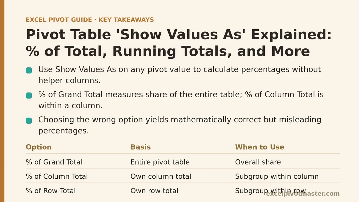
This turns each cell into a percentage of the single overall total across the entire pivot table, no matter how your data is broken out by rows or columns. Show regional sales this way, and every region’s percentage will add up to 100% across the whole table — not within any subgroup, but across everything.
Worth using when: you want an item’s share of the absolute overall total, with no further breakdown by any other dimension.
% of Column Total and % of Row Total
These calculate percentages against a subset instead of the grand total. % of Column Total turns each value into a percentage of its own column’s total — handy when years sit across the columns and you want each region’s share within one particular year. % of Row Total does the same thing, just across each row.
The mistake this catches people on: picking % of Grand Total when what you actually needed was % of Column Total gives you numbers that are mathematically sound but answer a different question than the one you asked. Every percentage will come out smaller than it should, because it’s being weighed against the whole table’s total instead of the specific column or row you care about.
How to tell which one you need: ask yourself plainly whether you want a value’s share of everything in the table, or its share inside one specific column or row grouping. If a percentage looks smaller than you’d expect, this mismatch is the first thing worth checking.
% of Parent Row Total and % of Parent Column Total
These earn their keep when your pivot table has nested row or column groupings — Region nested under Country, say. Instead of calculating against the grand total or the outermost row or column, these measure each value against its immediate parent grouping: a city’s percentage of its own region, not of the entire country.
Worth using when: you’re working with a multi-level hierarchy and want each level’s percentage to reflect its share of its own direct parent, rather than of the table as a whole.
Running Total In
This builds a cumulative sum as you move down through your data in a field’s specified order — each row’s value stacked on top of everything above it. It’s the right tool for tracking cumulative totals over time, cumulative sales by month being the classic case.
The order-dependency trap: Running Total In only works if your data is already sorted the way you want it accumulated. Months out of chronological order in your pivot table mean your “running total” accumulates in whatever order they happen to appear, and the resulting cumulative figure won’t represent what you meant to show.
How to confirm this is set up correctly: before trusting a running total, check explicitly that the field driving the accumulation — usually a date or sequence field — is sorted the way you intend, rather than assuming Excel has already handled that for you.
% Difference From and Difference From
These compare each value against a base item or field you select — most often a prior period, for period-over-period change.
The base-field trap that catches almost everyone: setting this up means choosing a Base Field and a Base Item in the dialog. Select “(previous)” as the base item, and the comparison shifts dynamically against whatever comes immediately before each item in the field’s order. Select one fixed item instead — a specific baseline year, for instance — and every other value gets compared against that single fixed point rather than against its own predecessor.
The two setups produce meaningfully different results, and choosing the wrong one for what you meant to compare is the most frequent error with this feature. One workshop participant was trying to compare “this year vs. last year” and accidentally selected a single fixed base year instead of “(previous).” Every subsequent year ended up measured against that one original year, not the year right before it.
How to confirm this is the cause: if percentages for later periods look unexpectedly large or off, check whether the Base Item is set to “(previous)” or to one fixed item — that single setting decides what every other value is being measured against.
Rank Largest to Smallest and Rank Smallest to Largest
Instead of a raw value or a percentage, these show each item’s rank relative to the others in your chosen base field — a fast way to spot top or bottom performers without manually sorting and counting.
Worth using when: the point you’re making is about relative standing — top performer, bottom performer — rather than the underlying number itself, especially on a dashboard where rank tells the story faster than raw figures would.
A Quick Reference for Choosing the Right Option
| What You Want to Know | Use This Option |
|---|---|
| Each item’s share of the entire table’s total | % of Grand Total |
| Each item’s share within its specific column or row group | % of Column Total / % of Row Total |
| Each item’s share within its immediate parent in a hierarchy | % of Parent Row/Column Total |
| Cumulative total building up over a sorted sequence | Running Total In |
| Change relative to the previous period specifically | % Difference From, Base Item = “(previous)” |
| Change relative to one fixed baseline period | % Difference From, Base Item = that specific period |
| Relative standing among categories | Rank Largest to Smallest / Smallest to Largest |
The Habit Worth Building
Before touching any Show Values As option, name the actual question you’re trying to answer: share of the whole table, share of one specific group, change from the period right before this one, or change from a single fixed baseline. Matching that question to its corresponding option — instead of grabbing whichever one sounds close and hoping the numbers look reasonable afterward — is what separates a quick, correct setup from the kind of manual rebuilding that workshop participant had been stuck doing for weeks.
What comparison or percentage are you trying to show in your pivot table? Describe what you want each value measured against, and I can tell you exactly which Show Values As option fits your case.
Related guides: 3 Ways to Summarize Pivot Table Values by Average, Median, and Mode, Excel Pivot Table Calculated Fields Explained: A Practical Guide, and Excel Pivot Table Layout Styles: Compact vs Outline vs Tabular Explained.