A blank row or a zero in a pivot table is often treated as a rendering glitch — something a quick Refresh or a re-sort will clear up. That assumption is wrong, and it costs people time. In most cases the blank is telling you something specific: a source cell is empty, a cache is holding an item that no longer exists, a layout setting is hiding labels, or a calculation is summing values that were never entered. Each cause produces a slightly different pattern of blanks, and each one needs a different fix. Treating them all as “the pivot is broken” means you will keep applying the wrong remedy and keep getting the same empty cells back.
The questions below follow the order readers tend to hit them: first the blank labels, then the zero totals, then the subtler cases. Find the question that matches your screen, apply the fix, and move on. Numbers cited here are typical ranges from how Excel generally behaves on ordinary datasets, not measurements of any specific workbook.
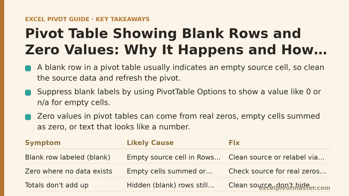
Why does my pivot table show a row labeled “(blank)”?
This is the most common complaint and the easiest to misdiagnose. The “(blank)” row appears when one or more rows in your source data have an empty cell in a field you placed in the Rows area.
Cause: Excel does not drop empty records from a pivot table. If your source has 1,000 rows and 14 of them have nothing in the Region column, the pivot creates a “(blank)” row to hold those 14 records and their related values. That is by design — the alternative would be silently losing data, which is worse.
Fix, if the blanks are true data errors: Clean the source. Go back to the source sheet, filter the relevant column for blanks, and either fill them with the correct value or delete the rows entirely. Refresh the pivot afterward. The “(blank)” row disappears once no source row is empty in that field.
Fix, if you want to suppress the label without touching the data: Right-click the pivot table → PivotTable Options → Layout & Format tab → tick For empty cells show and enter a value such as 0 or n/a in the box. This does not remove the row — it relabels it — but it stops the report from looking unfinished.
What not to do: Applying a label filter to hide “(blank)” looks like a fix and is not. The hidden records still exist and still contribute to your grand total, so the displayed rows will not add up to the displayed sum. That mismatch is the one readers notice first.
Why does my pivot table show zeros in cells where the source has no data?
Zero values and blank cells are not the same thing, and the difference matters for totals.
Cause A — the source cell contains a real zero. If a sales rep recorded 0 units for the month, the pivot shows 0. That is correct output.
Cause B — the cell is empty and the pivot is summing. Many Excel versions default to showing a zero for a sum over empty or non-numeric cells. An empty text cell contributes nothing to a SUM, but the pivot’s number formatting may display the absent result as 0.
Cause C — the source cell holds text that looks like a number. This is the trap that causes the most real damage. A cell containing "1,200" or "N/A" or " 350" with a leading space counts as text to Excel. The pivot treats it as non-numeric, contributes zero to any SUM, and shows 0 in the total. You look at the source, you see numbers, and the pivot disagrees — because the cells are text.
How to check for text-as-number: Select the source column and look at the status bar at the bottom of the window. If it shows a Sum and an Average, the column is numeric. If it shows only a Count, the column contains text. You can also turn on the Error Checking green triangle (Formulas → Error Checking → options) — text-formatted numbers often trigger it.
Fix: Convert the text back to real numbers. Select the column, then use Data → Text to Columns → Finish, which forces a re-parse, or use Paste Special → Multiply by 1 on a helper column. Refresh the pivot afterward.
Why do blank cells appear where I expect repeated labels, like a merged column?
This is a layout setting, not a data problem, and it confuses readers more than any other blank pattern.
Cause: With the Tabular Form layout and Repeat All Item Labels setting turned off, Excel suppresses a row label when it duplicates the row above. So a table of Region → City → Sales shows “North” once, then blank under it for every subsequent North city, rather than repeating “North” every row. Paste that into a report and the blanks look like missing data.
| Layout behavior | How row labels display | When to prefer it |
|---|---|---|
| Compact Form | All fields merged into one indented column | Dark, narrow screens; quick reading |
| Outline Form | Fields in separate columns, labels repeated in the leftmost only | On-screen analysis of two-level hierarchies |
| Tabular Form + Repeat All Item Labels | Every label repeated in every row | Copying into reports, or pivoting further downstream |
| Tabular Form without repeat | Labels shown once per group, blanks beneath | Compact printing; careful readers only |
Fix: Go to Design → Layout → Report Layout → Show in Tabular Form. Then Design → Layout → Repeat All Item Labels. The blanks fill in and the table becomes copy-and-paste safe.
Why do I get a zero grand total when the individual values look correct?
This one is worth slowing down on, because the pivot is usually right and the source is wrong in a specific way.
Cause 1 — the values column is pointed at text. If the sum field references a column where most entries are text, every one of those entries contributes zero. The visible rows where a number did get parsed look fine; the total is far too low or flat zero because the rest did not count. Confirm by pulling the source column into a =SUM() cell in a spare corner — if SUM returns 0 but COUNT returns a large number, the column is text.
Cause 2 — the number format is rounding to zero. A column formatted as Currency with zero decimals will display $0 for 0.40. Right-click the values field → Field Settings → Number Format and check the decimal places. Formatting also affects the total.
Cause 3 — the filter on the pivot is excluding the rows that would contribute. Look at the field dropdowns. An active filter hidden in a pivot table is easy to miss, especially after a save-and-reopen cycle.
Cause 4 — the workbook has automatic calculation turned off. Formulas → Calculation Options → Automatic. In manual mode, source changes are not carried into the pivot until you force a recalculation and refresh.
Why do blank or zero rows appear even after I press Refresh?
When a refresh fails to fix the blanks, the cache is usually the reason.
Blank row that should have been deleted: The pivot cache is retaining items that no longer exist in the source. Rows you deleted from the source still appear as blank or zero rows after a refresh. This is the cache’s item-retention behavior. Set Number of items to retain per field to None (PivotTable Options → Data), then refresh. The orphan items clear.
Zero rows that reflect an outdated range: The pivot cache points at a fixed range, so source data added below that range is not read. Extend the source range via Change Data Source, or — better — convert the source to an Excel Table (Ctrl+T) and rebuild the pivot on the Table name so it grows automatically.
Blank cell that should have a value: If the source cell was edited after the last refresh, the pivot still holds the old cached value. Confirm by checking the Last refreshed timestamp under PivotTable Options → Data. If it predates your edit, you have not refreshed since making it.
Why do my GETPIVOTDATA formulas return blanks or zeros?
If formulas outside the pivot table pull from it using GETPIVOTDATA (the automatic behavior when you click a pivot cell while writing a formula), any change to the pivot’s layout can break them silently.
Cause 1 — the field or item name changed. GETPIVOTDATA matches against exact item names. If you renamed a region, changed the column label, or removed an item, the formula returns #REF! or, in some configurations, zero.
Cause 2 — the pivot layout changed. Switching from Tabular to Compact form, or moving a field between Areas, can invalidate the field references in the formula.
Cause 3 — the reference points at a cell outside the current pivot. If the pivot shrank because items were removed, the referenced cell may no longer contain data.
Fix: Rewrite the GETPIVOTDATA using the actual field names from the new layout, or replace it with a plain cell reference if the pivot’s shape is stable. If you use these formulas extensively, wrap them in IFERROR so a broken reference shows a clear label rather than a bare zero that looks like real data.
What blank and zero symptoms tell you, at a glance
| Symptom on screen | Most likely cause | Fix |
|---|---|---|
| Row labeled “(blank)” | Empty cells in a source field | Fill or delete the empty source rows |
| Zero cells where source has no value | Text-as-number in the source column | Convert the column to numeric |
| Blank repeated labels | Tabular form without Repeat All Item Labels | Turn on Repeat All Item Labels |
| Deleted categories still appearing as blank/zero rows | Cache retaining old items | Set retain items to None, then refresh |
| Grand total far below expected | Values field pointing at a text column | Check with =SUM() vs =COUNT() on the source |
| All values zero after reopening the file | Automatic calculation off, or stale cache | Set calculation to Automatic, refresh |
The mistakes that make blank-and-zero problems worse
- Hiding blanks with a filter. The records survive and still count toward totals. You trade one visible problem for a total that does not sum.
- Pasting the pivot’s values into a report while blanks are suppressed. Copying only the visible cells means the pasted numbers will not foot. Turn on Repeat All Item Labels before copying.
- Converting a text-as-number column with Find & Replace. Replacing commas or spaces individually rarely works cleanly on large ranges. Text to Columns or Paste Special → Multiply is faster and more consistent.
- Rebuilding the pivot before checking the source. If the source has empty or text cells, a fresh pivot built on it will show the same blanks and zeros. Fix the source first.
- Forgetting to refresh after changing a cache setting. The retain-items and layout settings apply on the next refresh, not immediately.
What to check in the next ten minutes
Open the workbook with the blank or zero problem and work down this list:
- Count the blanks. Filter the Rows-area source column for
(Blanks). If the count is more than a handful, clean the source instead of masking the symptom. - Test the values column. In a spare cell, enter
=SUM()over the source column the pivot is summing. If it returns 0 and=COUNT()returns a large number, the column is text — convert it. - Check the layout. Design → Report Layout → Show in Tabular Form, then Repeat All Item Labels, if you plan to copy the output anywhere.
- Set retain-items to None if any deleted rows are still appearing. Then refresh and confirm the orphans are gone.
- Reconcile one number by hand. Pick a single row, sum its source records, and compare to the pivot. A mismatch points at a remaining blank, zero, or stale-cache issue.
If the blanks persist after all five checks, note which row on the symptom table above matches what you see — that pairing narrows the cause to one or two possibilities faster than rechecking settings you have already ruled out.
Related guides: Pivot Table Not Refreshing: Common Causes and Fixes, Fixing Pivot Table Refresh Errors and Stale Data Problems, and Pivot Table Not Showing All Data: Fix Guide for Every Cause.