A pivot table’s grand total is not the sum of the visible numbers when a filter is applied the wrong way — it is the sum of everything the cache still holds. That single fact explains most of the refresh problems people run into, and it is also the reason Power Query’s Group By feature is worth learning even if you already know pivot tables well. Group By does not summarize on screen. It rewrites the data into a new table that contains only the summarized rows, and that table becomes your source.
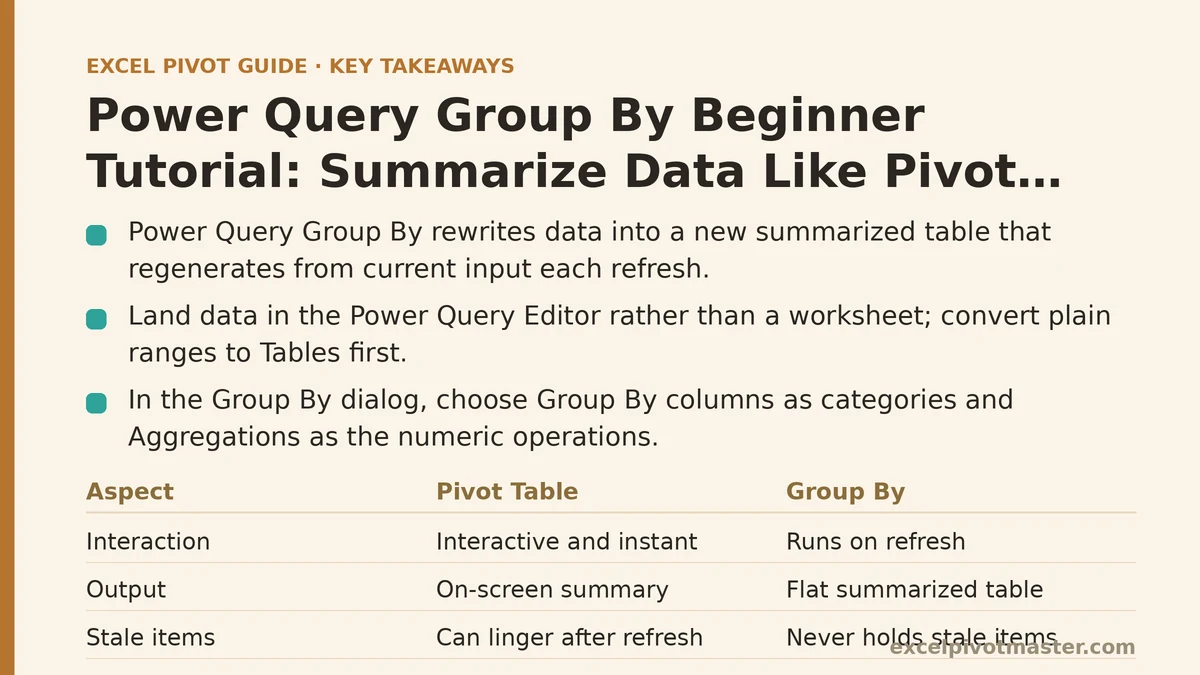
The trade is straightforward. A pivot table is interactive and instant. A Group By step is a transformation that runs on refresh, produces a flat table, and never holds stale items because there is nothing to hold — the output is regenerated from the current input every time. For anyone who has watched a deleted region linger in row labels after a refresh, that distinction matters more than the extra setup.
This tutorial walks through the whole thing in sequence, from loading a range to reading the generated M code.
Step 1: Get Your Data Into Power Query
Before any grouping happens, the source has to be somewhere Power Query can read it. Three common starting points:
- An Excel Table (Ctrl+T). Select any cell in the table, then go to Data → Get & Transform Data → From Table/Range. This is the cleanest option because the table expands automatically as rows are added, and the query follows the table name rather than a fixed cell address.
- A CSV or text file. Data → Get Data → From File → From Text/CSV. Choose the file, then in the preview dialog click Transform Data rather than Load. Transform Data opens the Power Query Editor; Load would import the raw file straight into a worksheet without giving you a place to add the Group By step.
- A folder of files. Data → Get Data → From File → From Folder. Useful when monthly exports arrive as separate files, but heavier than what a first Group By exercise needs.
One rule applies to all three: land in the Power Query Editor, not directly in a worksheet. The Editor is where every subsequent step gets recorded.
If you are working from a plain range rather than a Table, convert it first. Building a query on a fixed range reintroduces the same stale-range problem that Group By is meant to remove.
Step 2: Decide What Goes in “Group By” and What Gets Aggregated
The Group By dialog asks for two things, and the split between them is the only real design decision in this whole process:
- Group By columns — the categories you would put in a pivot table’s Rows area. Region, Product, Salesperson, Month. Each unique combination of these becomes one row in the output.
- Aggregations — the numbers you would put in the Values area. A column, an operation (Sum, Count, Average, Min, Max, Median), and an output name.
A pivot table asks the same question with drag-and-drop. Region in Rows, Sales in Values, done. Group By asks it with a dialog and writes the result into the data itself.
Two practical notes before you click anything:
Order the Group By columns deliberately. Region followed by Product produces a two-level grouping. Product followed by Region produces the same totals in a different sort order and a different visual shape. Neither is wrong; pick the one that matches how the report will be read.
Name your output columns at this stage. Power Query will suggest names like “Sum of Sales” and “Count of OrderID.” Accepting them is fine, but if the downstream report needs “Total Revenue,” type that in the output field now. Renaming later means editing the M code or adding a Rename Columns step, both of which are extra work for no benefit.
Step 3: Run the Group By
With the query open in the Power Query Editor:
- Go to the Home tab and click Group By. It sits in the Transform group, roughly a third of the way along the ribbon.
- In the dialog, choose Basic mode for a first pass. Advanced mode lets you add multiple aggregations in one step — useful later, unnecessary now.
- Pick your Group By columns from the dropdown. If you need more than one, click Add grouping and select another.
- Click Add aggregation, then set the new column name, the operation, and the source column for each summary you want.
- Click OK.
The preview pane on the right updates immediately. Where the table previously showed every transaction row, it now shows one row per unique combination of your grouping columns, with the aggregated values beside them.
If the row count drops from thousands to a few dozen, the grouping worked. If it barely changes, your Group By columns are too granular — grouping by OrderID alongside Region, for example, produces roughly one output row per input row because each order is already unique.
Step 4: Check the One Behavior That Catches Beginners
Right-click any aggregated value in the preview and look at what you get: a static number, not a formula. There is no SUM() anywhere in the output. The aggregation happened once, during the query’s evaluation, and the result was written as a value.
This is the core difference from a pivot table, and it has a consequence worth understanding before you build on it.
A pivot table recalculates its aggregation against the cached range on every refresh. A Group By step re-runs the entire query from the source on every refresh, which means it re-reads the full input, re-applies every prior step (filtering, type changes, column removal), and re-computes every aggregation from scratch. On a few thousand rows that is imperceptible. On a hundred thousand rows it may add a visible pause each time the workbook opens or the query is refreshed.
The practical upshot: Group By is not a replacement for pivot tables in interactive work. It is a replacement for pivot tables in report pipelines — situations where the summarized shape is what you want to hand to a chart, a dashboard, or another worksheet, and where you want that shape to be reproducible rather than manually refreshed.
Step 5: Load the Result and Read the Generated M
Click Close & Load (or Close & Load To… to send the output to a specific worksheet or the Data Model). Excel writes the summarized table into a new worksheet and registers the query in the Queries & Connections pane.
Now open the Advanced Editor under the View tab. The Group By step you clicked through is now a block of M code, and it looks roughly like this:
= Table.Group(#"Changed Type", {"Region", "Product"}, {
    {"Total Sales", each List.Sum([Sales]), type number},
    {"Orders", each Table.RowCount(_), Int64.Type}
})
Three things are visible here that are not obvious from the dialog:
#"Changed Type"is the name of the previous step. Group By operates on whatever the step before it produced, not on the original file. If an earlier step filtered out rows or removed a column, that is already reflected.{"Region", "Product"}is the list of grouping columns.- Each
{...}inside the list is one aggregation: a new column name, a function (List.Sum,Table.RowCount), and a type.
You do not need to write M to use Group By. But reading this block once explains why reordering your steps matters — if you insert a filter after the Group By step, the filter applies to the already-summarized rows, not to the underlying transactions. That single misordering produces wrong totals that look plausible, which is the worst kind of wrong.
Step 6: When the Source Changes, Refresh
Here is where Group By earns its place. Update the source table, add a new region, delete a discontinued product line, and then press Data → Refresh All (or Ctrl+Alt+F5).
The query re-runs from the top. Any new region appears in the output as a new row with its own totals. Any deleted product disappears, along with its rows. There is no orphan-item problem, because the summarized table is not a view over a cache — it is the result of a computation that gets thrown away and rebuilt each time.
Two settings worth confirming on a Pipeline you intend to share:
- Refresh on open. In the Queries & Connections pane, right-click the query → Properties → Usage, and tick “Refresh data when opening the file.” Without it, a colleague opening the workbook sees the last-loaded output, which is the same staleness trap a pivot table falls into.
- Refresh in background. Leave the default on for small sources; turn it off for very large ones so the load happens predictably rather than mid-session.
Common Mistakes and How to Recover
Grouping on the wrong columns. If the output has more rows than expected, you grouped by something nearly unique — a date, an ID, an order number. Remove the offending column from the Group By list rather than adding a filter downstream.
Aggregating a text column. Sum, Average, and Median need numbers. If the column has mixed types, Power Query may have typed it as text. Go back to the Changed Type step, or add one, and set the column to a numeric type before grouping.
Putting a filter after the Group By step. Filters belong before Group By in almost every case. The exception is filtering on the aggregated values themselves — “show only products with total sales above 10,000” — which correctly belongs after.
Re-running Group By twice by accident. Applying Group By to an already-summarized table sums the sums. Unless the query feeds into a deliberately staged pipeline, group once and stop.
Forgetting to rename the output. “Sum of Sales” is fine for a scratch query. It is not fine for a column a chart or a second query references by name. Rename at the Group By dialog, or add a Rename Columns step immediately after.
Group By vs. Pivot Table: Choosing per Task
| Situation | Better fit |
|---|---|
| Interactive exploration, changing layout on the fly | Pivot table |
| Fixed report shape that must refresh identically for every user | Power Query Group By |
| Multiple pivots that must stay in sync | Group By feeds all of them |
| Source data with rows frequently deleted | Group By, to avoid the stale-item trap |
| Very large source, refreshed often | Pivot table, unless the query is engineered carefully |
| Output feeding a chart or a second query by column name | Group By |
The two are not in competition. A common pattern is to use Group By in Power Query to produce a clean summarized table, then build a pivot table on top of that output for interactivity. The pivot is fed by data that has already been reduced to a manageable size, and the Group By handles the part that pivot tables handle badly — keeping deleted categories from lingering.
What to Do Next
Pick one report where a pivot table has served stale numbers, or where a colleague has asked for “the same numbers as last month but current.” Run through this sequence on it today:
- Convert the source to an Excel Table and load it into Power Query via Data → From Table/Range.
- Add a Group By step with your category columns and one Sum aggregation.
- Load the output to a new worksheet, then change one row in the source and hit Refresh All to confirm the output follows.
- Tick Refresh on open in the query’s properties if the file is shared.
The whole sequence takes about five minutes on a small source. What you get back is a summary that rebuilds itself from the data every time it runs, with no cache to go stale and no orphan categories to remove by hand.
Related guides: Power Query Unpivot Columns: A Beginner Tutorial for Pivot-Ready Data, Power Query vs Pivot Tables: When to Use Each (Ranked by Task), and Pivot Table vs Power Query: When to Use Which.