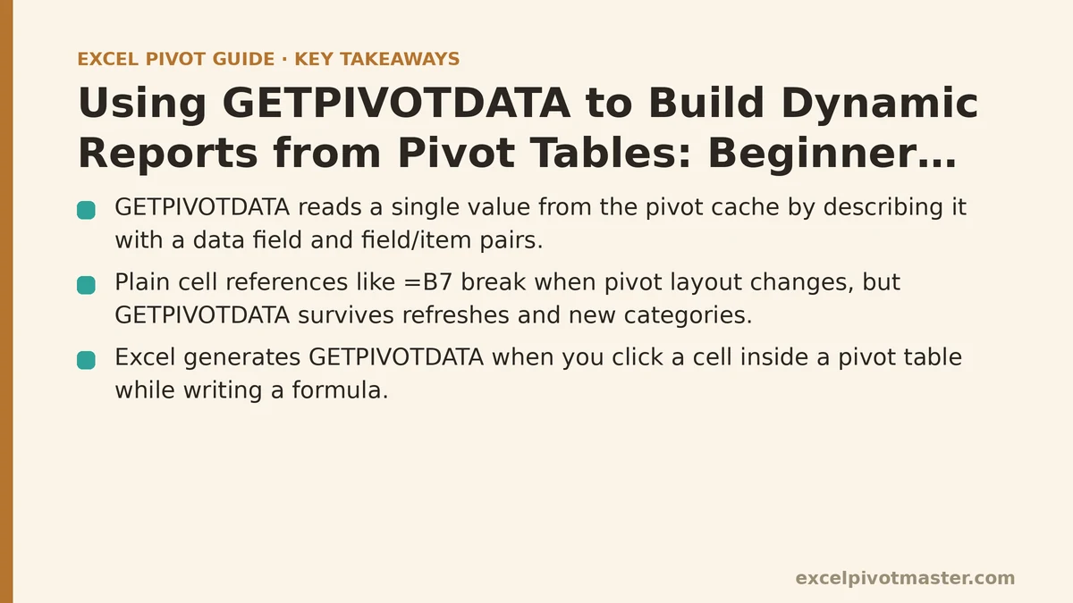
Clicking a cell inside a pivot table while writing a formula produces a result many people find alarming. Instead of =B7, Excel inserts something long and strange like =GETPIVOTDATA("Sales",$A$3,"Region","North"). Most users immediately delete it and hunt for a way to turn the feature off, because the syntax looks unreadable and it seems to do the same job as a plain cell reference.
That instinct is usually a mistake. The plain reference =B7 breaks the moment the pivot table’s layout shifts — a new region appears and everything slides down a row, or you collapse one field and the cell you were pointing at now holds a different number entirely. The long formula keeps working because it addresses the data by name rather than by position. Once you understand its four parts, you can build report sheets that stay correct through refreshes, layout changes, and new categories.
This tutorial walks through GETPIVOTDATA from the ground up: what each argument does, how to write the function by hand, where it fails, and how to assemble a small dashboard that survives real use.
Step 1: Understand What GETPIVOTDATA Is Retrieving
Every pivot table stores its results in a hidden structure called the pivot cache — a snapshot of the source data organized by the field combinations you dropped into the Rows, Columns, Filters, and Values areas. GETPIVOTDATA reads a single value out of that cache by describing it: a data field, plus the field/item pairs that locate one cell in the grid.
The function has this shape:
=GETPIVOTDATA(data_field, pivot_table, [field1, item1], [field2, item2], ...)
- data_field — the name of the value field you want, wrapped in quotes, such as
"Sum of Sales"or"Count of Orders". This matches the header Excel shows in the Values area, not necessarily the source column name. - pivot_table — any cell inside the pivot table. Commonly written as
$A$3, the top-left corner of the pivot’s output range. - field / item pairs — the row, column, and filter fields that pinpoint the value, written as
"Region","North","Month","Jan", and so on.
The breakthrough for most people is realizing the pairs are optional in count but not in kind. Supply one pair and you get the value for that single condition, provided it uniquely identifies a cell. Supply two and you narrow to an intersection. Omit them entirely and you get the grand total.
Step 2: Generate Your First Formula by Pointing and Clicking
The fastest way to learn the syntax is to let Excel write it for you, then read what it produced.
- Click a blank cell outside the pivot table — a report cell, not part of the pivot itself.
- Type
=to begin a formula. - Click a single data cell inside the pivot table — for example, the intersection of the “North” row and the “Jan” column in a Sales grid.
- Press Enter.
The formula bar now shows something like:
=GETPIVOTDATA("Sales",$A$3,"Region","North","Month","Jan")
Read it back in plain language: “from the pivot table starting at A3, give me the Sales value where Region is North and Month is Jan.” The two field/item pairs match the two labels that defined the cell you clicked. If your pivot has a filter field applied, a third pair for that filter may also appear.
If clicking inside the pivot table gives you an ordinary =B7 reference instead, the generation feature is switched off. Turn it on via PivotTable Analyze → Options → Generate GetPivotData. When the toggle is on, Excel writes the function automatically; when off, it writes cell references. Both work, but only one survives layout changes.
Step 3: Write the Formula by Hand for a Fixed Report Cell
Point-and-click is fine for a one-off, but a report sheet usually needs the same figure in a specific spot regardless of where the pivot places it. Writing the function manually gives you that control, and it is easier than the length of the string suggests.
Suppose your pivot table starts at cell A3, its row field is Region, its column field is Month, and its value field is Sum of Sales. To place January’s North figure in cell H2 of a report sheet:
=GETPIVOTDATA("Sum of Sales",$A$3,"Region","North","Month","Jan")
Two habits make these formulas far easier to maintain:
- Anchor the pivot_table argument with absolute references (
$A$3, notA3). If you copy the formula down a column, a relative reference would drift and start pointing outside the pivot, producing a#REF!error. - Match the field and item text exactly. Field names and item labels are case-insensitive and tolerate extra spaces, but “Jan” will not match a source value stored as “January”. The label must match what the pivot displays.
Step 4: Replace Hard-Coded Labels with Cell References
Typing "North" and "Jan" directly into the formula works, but it defeats the purpose of a dynamic report. Instead, let the formula read those labels from cells you control, so changing a dropdown or a cell value re-points the whole report without editing any formula.
Set up a small input area — say cell J1 holds a region name and J2 holds a month — then write:
=GETPIVOTDATA("Sum of Sales",$A$3,"Region",$J$1,"Month",$J$2)
Now the report cell always shows the figure for whichever region and month are typed in J1 and J2. Change J1 to “South” and the number updates instantly. This is the core technique behind nearly every dynamic pivot report: the pivot table holds all the combinations, and GETPIVOTDATA extracts the one the user selects.
A useful pairing here is a data validation dropdown on J1 and J2, populated from the same list the pivot uses. That way a reader can never type a label the pivot does not recognize, which is the single most common source of #REF! errors.
Step 5: Pull Totals, Subtotals, and Grand Totals
GETPIVOTDATA handles aggregate rows the same way it handles detail cells — by loosening the number of field/item pairs.
- Grand total across everything: omit every pair.
=GETPIVOTDATA("Sum of Sales",$A$3)returns the overall total. - Total for one region: supply only the row field pair.
=GETPIVOTDATA("Sum of Sales",$A$3,"Region","North")returns North’s total across all months. - Total for one month: supply only the column field pair.
=GETPIVOTDATA("Sum of Sales",$A$3,"Month","Jan")returns January’s total across all regions.
The rule to remember: whatever combination you leave out is aggregated. Leaving out the Month pair sums every month together; leaving out both sums everything. This is why the same function can populate a KPI cell at the top of a dashboard and a specific intersection further down, without two different techniques.
One detail worth knowing: the total returned reflects the pivot table’s own totals, including any filters currently applied to the pivot. If someone collapses a field or applies a report filter, the figure changes. That is usually what you want, but it means a GETPIVOTDATA total is not the same thing as an unfiltered sum of the raw source column.
Step 6: Diagnose the Most Common GETPIVOTDATA Errors
The function has a small set of failure modes, and each has a specific cause and fix.
#REF! on every recalculation, or the formula returns nothing. This almost always means a field name or item label no longer matches the pivot. Common triggers: a source value was renamed from “North” to “Northern”, a value was deleted so “East” no longer exists as a category, or the pivot was reconfigured so a field that used to be in Rows moved to Columns. Open the pivot’s field list, compare the exact text of each field and item, and correct the formula to match.
#REF! right after copying the formula. An unanchored pivot_table argument drifted relative to the new location. Change $A$3 to absolute references.
The formula returns a value for a category that no longer appears in the source data. The pivot cache is retaining stale items. Set PivotTable Options → Data → “Number of items to retain per field” to None, then refresh, and the orphan label disappears — along with the formula that depended on it.
The result refuses to update after new data is added. The pivot table itself needs a refresh; GETPIVOTDATA reads the cache, not the raw sheet. Press Ctrl+Alt+F5 to refresh every pivot in the workbook, or refresh the single table via right-click → Refresh. The formulas follow automatically.
The value field name does not match the source column. Value fields carry a prefix in the pivot — “Sum of Sales”, “Count of Orders”, “Average of Price”. The data_field argument must use that displayed name, prefix included. A formula written as GETPIVOTDATA("Sales",...) fails when the Values header reads “Sum of Sales”.
A quick diagnostic when a formula misbehaves: click the exact pivot cell you expect the formula to reproduce, then look at the formula Excel generates for that click. Comparing your hand-written version against the auto-generated one usually reveals the mismatched label or field in seconds.
Step 7: Assemble a Small Dynamic Report
With the pieces in place, a working report comes together quickly. This is the practical payoff of everything above.
The setup. A pivot table at A3 summarizing Sum of Sales by Region (rows) and Month (columns), sourced from an Excel Table so it grows automatically. Two input cells for region and month, each backed by a dropdown. A grid of report cells beside the inputs.
The report cells. Each figure uses the same pattern, changing only the field/item pairs:
| Report cell shows | Formula pattern |
|---|---|
| Selected region, selected month | =GETPIVOTDATA("Sum of Sales",$A$3,"Region",$J$1,"Month",$J$2) |
| Selected region, all months | =GETPIVOTDATA("Sum of Sales",$A$3,"Region",$J$1) |
| All regions, selected month | =GETPIVOTDATA("Sum of Sales",$A$3,"Month",$J$2) |
| Overall total | =GETPIVOTDATA("Sum of Sales",$A$3) |
| Selected region’s share of total | =GETPIVOTDATA("Sum of Sales",$A$3,"Region",$J$1)/GETPIVOTDATA("Sum of Sales",$A$3) |
Adding a comparison. Because these are ordinary formulas, you can nest them inside other functions. A percentage-of-total, a variance against a prior period, or a threshold flag all work by wrapping two GETPIVOTDATA calls in arithmetic. A cell formatted as a percentage showing selected-region share is simply the fourth row above, with the cell number formatted as 0.0%.
The refresh behavior. When the source data changes, one refresh updates the pivot, and every report cell recalculates from the new cache. Nothing on the report sheet needs editing — provided the labels in the input cells still exist as categories in the data.
Step 8: Decide Whether GETPIVOTDATA Is the Right Tool
It solves a specific problem, and it is not always the right answer.
| Situation | GETPIVOTDATA fits? | Better approach |
|---|---|---|
| A fixed set of report cells must survive pivot layout changes | Yes | — |
| A dashboard pulls figures for a user-selected category | Yes | — |
| You need a plain cell offset that never moves | Rarely | Use a normal =B7 reference |
| The value does not come from a pivot at all | No | Use SUMIFS or XLOOKUP on the source table |
| You only need the number once, in place, with no reuse | Either works | A cell reference is simpler |
The honest trade-off: GETPIVOTDATA formulas are long, unforgiving of typos in labels, and confusing to anyone who opens the workbook cold. A plain reference is short but fragile. For a report that will be refreshed and reused, the fragility is the bigger risk, and the long formula earns its keep. For a throwaway calculation, skip it.
What to Do Next
Open a workbook that contains a pivot table you refresh regularly, and build the smallest possible dynamic report on it, today:
- Generate one formula by pointing at a single data cell to confirm Generate GetPivotData is on, then delete it and retype the same logic by hand.
- Add two input cells for a row label and a column label, with data validation dropdowns fed from the same categories the pivot uses.
- Write one dynamic formula that reads both inputs, and confirm it updates when you change either dropdown.
- Add a total cell using the pair-omission rule from Step 5, and a share-of-total cell dividing the two.
- Refresh the pivot once (Ctrl+Alt+F5) and watch the report cells follow.
If any formula returns #REF!, compare it against the auto-generated version for the same cell — the mismatch is nearly always a label or field name that no longer matches the pivot’s current item list. Fix that one string and the report comes back to life.
Related guides: How to Combine Pivot Tables with VLOOKUP and INDEX/MATCH, Why Does GETPIVOTDATA Keep Appearing in My Formulas? (And How to Turn It Off), and GETPIVOTDATA Function Beginner Tutorial: Extract Pivot Data.